40 excel chart remove 0 data labels
Graphs - remove data labels and category name when Zero Jan 9, 2012. #1. I am creating a pie graph. This graph contains % of business areas which meet certain criteria. Some business areas meet 0%. I dont want to see those that are 0%, I know I can go to number format and use this custom format: 0%;;; This gets rid of the 0's. However, it does not get rid of the Business area category name. Add or remove data labels in a chart VerkkoRemove data labels from a chart. Click the chart from which you want to remove ... For example, if you calculate 10 / 100 = 0.1, and then format 0.1 as a percentage, the number will be correctly ... You can add data labels to show the data point values from the Excel sheet in the chart. This step applies to Word for Mac only: On the View menu ...
What Are Data Labels in Excel (Uses & Modifications) - ExcelDemy Click on the Add Chart Element under Chart Layouts, select Data Labels, and next choose None. By clicking the data label once, you can select all data labels, or you can click the label twice to select only one of the data labels you wish to delete, and finally, you can press the DELETE button.

Excel chart remove 0 data labels
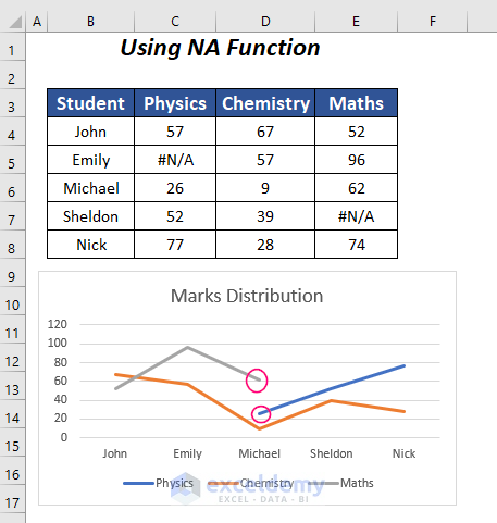
Creating a chart in Excel that ignores #N/A or blank cells VerkkoI am attempting to create a chart with a dynamic data series. Each series in the chart comes from an absolute range, but only a certain amount of that range may have data, and the rest will be #N/A.. The problem is that the chart sticks all of the #N/A cells in as values instead of ignoring them. I have worked around it by using named dynamic … How to rotate axis labels in chart in Excel? - ExtendOffice VerkkoRotate axis labels in Excel 2007/2010. 1. Right click at the axis you want to rotate its labels, select Format Axis from the context menu. See screenshot: 2. In the Format Axis dialog, click Alignment tab and go to the Text Layout section to select the direction you need from the list box of Text direction. See screenshot: 3. Legends in Chart | How To Add and Remove Legends In Excel Chart… A Legend is a representation of legend keys or entries on the plotted area of a chart or graph, which are linked to the data table of the chart or graph. By default, it may show on the bottom or right side of the chart. The data in a chart is organized with a combination of Series and Categories. Select the chart and choose filter then you will ...
Excel chart remove 0 data labels. How can I hide 0% value in data labels in an Excel Bar Chart The quick and easy way to accomplish this is to custom format your data label. Select a data label. Right click and select Format Data Labels; Choose the Number category in the Format Data Labels dialog box. How to hide zero in chart axis in Excel? - ExtendOffice 1. Right click at the axis you want to hide zero, and select Format Axis from the context menu. 2. In Format Axis dialog, click Number in left pane, and select Custom from Category list box, then type #"" in to Format Code text box, then click Add to add this code into Type list box. See screenshot: Hiding zero values in Excel chart or diagram, legend and ... 12 Jun 2017 · 1 answerRight click at one of the data labels, and select Format Data Labels from the context menu · In the Format Data Labels dialog, Click Number in ... How to hide zero data labels in chart in Excel? - ExtendOffice In the Format Data Labelsdialog, Click Numberin left pane, then selectCustom from the Categorylist box, and type #""into the Format Codetext box, and click Addbutton to add it to Typelist box. See screenshot: 3. Click Closebutton to close the dialog. Then you can see all zero data labels are hidden.
excel - How to not display labels in pie chart that are 0% - Stack Overflow 0 You don't show your data, so I will assume it is in column B, with category names in column A Generate a new column with the following formula: =IF (B2=0,"",A2) Then right click on the labels and choose "Format Data Labels" Check "Value From Cells", choosing the column with the formula and percentage of the Label Options. How to add data labels from different column in an Excel chart? VerkkoReuse Anything: Add the most used or complex formulas, charts and anything else to your favorites, and quickly reuse them in the future. More than 20 text features: Extract Number from Text String; Extract or Remove Part of Texts; Convert Numbers and Currencies to English Words. Merge Tools: Multiple Workbooks and Sheets into One; Merge Multiple … How to eliminate zero value labels in a pie chart However you can hide the 0% using custom number formatting. Right click the label and select Format Data Labels. Then select the Number tab and then Custom from the Categories. Enter. 0%; [White] [=0]General;General. in the Type box. This will set the font colour to white if a label has a value of zero. How to Use Cell Values for Excel Chart Labels Verkko12.3.2020 · Make your chart labels in Microsoft Excel dynamic by linking them to cell values. When the data changes, the chart labels automatically update. In this article, we explore how to make both your chart title and the chart data labels dynamic. We have the sample data below with product sales and the difference in last month’s sales.
How to make a histogram in Excel 2019, 2016, 2013 and 2010 - Ablebits.com Make a histogram using Excel's Analysis ToolPak. With the Analysis ToolPak enabled and bins specified, perform the following steps to create a histogram in your Excel sheet: On the Data tab, in the Analysis group, click the Data Analysis button. In the Data Analysis dialog, select Histogram and click OK. In the Histogram dialog window, do the ... How to suppress Category in Excel Pie Chart for zero values? 1. The data source for the Pie chart is Pivot table, with values set as % of column total. I am able to suppress the data values in the Pie chart by custom formatting number in Data labels, as #. But this still leaves Category name visible. Please advise how to suppress the Category name. excel. Chart label macro with toggle data labels on/off Hi all, I have this macro that works great for adding/deleting data labels. This worked perfectly before I added two new series (line chart). I want to modify below macro to just add/delete labels to series 1 and series 2 but I just can figure out how to write the syntax. Thanks for any... Data Labels in Excel Pivot Chart (Detailed Analysis) Click on the Plus sign right next to the Chart, then from the Data labels, click on the More Options. After that, in the Format Data Labels, click on the Value From Cells. And click on the Select Range. In the next step, select the range of cells B5:B11. Click OK after this.
How to Quickly Remove Zero Data Labels in Excel | by Ramin ...
Remove Chart Data Labels With Specific Value This VBA code will loop through all your chart's data points and delete any data labels that are equal to zero. Sub RemoveDataLabels_ByDeletion () 'PURPOSE: Delete Data Labels With a Values of 0. 'SOURCE: . Dim srs As Series. Dim x As Long.
Add / Move Data Labels in Charts – Excel & Google Sheets ...
How to Remove Zero Data Labels in Excel Graph (3 Easy Ways) 2 Aug 2022 — Steps: ➤ Select the dataset and then go to the Home Tab >> Editing Group >> Sort & Filter Dropdown >> Filter Option. Filter option.

Chart Elements in Excel VBA (Part 2) - Chart Series, Data ...
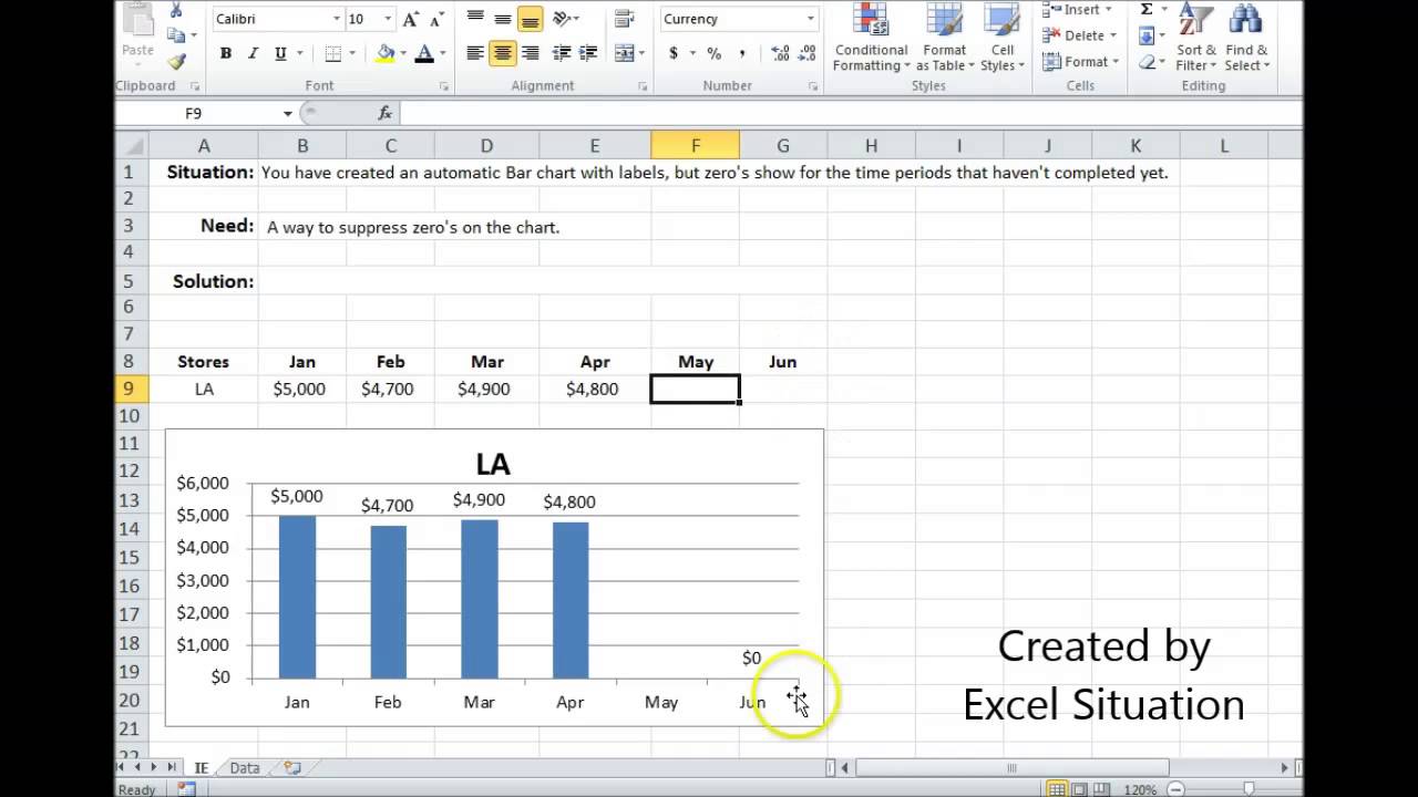
How to suppress 0 values in an Excel chart - TechRepublic You can hide the 0s by unchecking the worksheet display option called Show a zero in cells that have zero value. Here's how: Click the File tab and choose Options. In Excel 2007, click the Office...
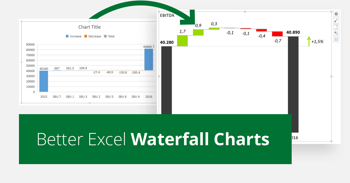
Excel Waterfall Chart: How to Create One That Doesn't Suck
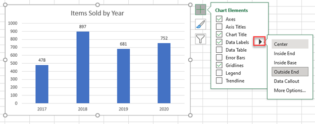
Edit titles or data labels in a chart - support.microsoft.com To edit the contents of a title, click the chart or axis title that you want to change. To edit the contents of a data label, click two times on the data label that you want to change. The first click selects the data labels for the whole data series, and the second click selects the individual data label. Click again to place the title or data ...

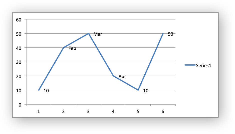
Directly Labeling Your Line Graphs | Depict Data Studio
Hide Series Data Label if Value is Zero - Peltier Tech Then apply custom number formats to show only the appropriate labels. In Number Formats in Excel I show how the number format provides formats for positive, negative, and zero values, and for text, with the individual formats separated by semicolons: ;;; Apply the following three number formats to the three sets of value data labels:

How to Customize Your Excel Pivot Chart Data Labels - dummies
Dynamically Label Excel Chart Series Lines • My Online ... Sep 26, 2017 · Hi Mynda – thanks for all your columns. You can use the Quick Layout function in Excel (Design tab of the chart) to do the labels to the right of the lines in the chart. Use Quick Layout 6. You may need to swap the columns and rows in your data for it to show. Then you simply modify the labels to show only the series name.

Display Customized Data Labels on Charts & Graphs
Remove zero data labels on chart - Excel Help Forum If using formulas, include condition to exhibit #N/A instead of zero. Over chart area, right button options, click Select Data. At dialog box, click Hidden and blank cells. At new dialog box, click Show data in hidden rows and columns. Not sure about precise English version for those commands, but they will show something like that. Godspeed!
libxlsxwriter: Working with Charts
Excel 2016 Chart Data Labels Always Empty - Stack Overflow The data labels object box is showing (I can also apply Fill and Border colors to it). However, this object is always EMPTY. Regardless of what I tick to show (e.g. Values, Values from Cells, Series Name, etc...) - it is always empty, with the minimum (shrunk) width (as it should expand per the value presented).
Add / Move Data Labels in Charts – Excel & Google Sheets ...
think-cell :: KB0195: How can I hide segment labels for If the chart is complex or the values will change in the future, an Excel data link (see Excel data links) can be used to automatically hide any labels when the value is zero ("0"). Open your data source. Use cell references to read the source data and apply the Excel IF function to replace the value "0" by the text "Zero". Create a think-cell ...

Solved: How to show all detailed data labels of pie chart ...
excel - Removing Data Labels with values of zero then reset - VBA ... activesheet.chartobjects ("chart 5").activate with activechart.seriescollection (1) for i = 1 to .points.count if .points (i).hasdatalabel = false then .points (i).select activechart.setelement (msoelementdatalabelshow) if .points (i).datalabel.text = 0 then .points (i).hasdatalabel = false .points (i).datalabel.showvalue = false end if …

Use drop down lists and named ranges to filter chart values
Column Chart with Primary and Secondary Axes - Peltier Tech Verkko28.10.2013 · Plot data in clustered column chart (Chart 1). Assign Sec 1 & Sec 2 to secondary axis (Chart 2). Set primary Y axis scale to 0 min and 6 max, set secondary Y axis scale to -30 min and +30 max (Chart 3). Use custom number format [<=3]0;;; for primary axis tick labels, use custom number format 0;;0; for secondary axis tick labels …
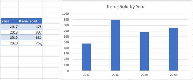
EXCEL Charts: Column, Bar, Pie and Line
How can I hide 0-value data labels in an Excel Chart? Right click on a label and select Format Data Labels. Go to Number and select Custom. Enter #"" as the custom number format. Repeat for the other series labels. Zeros will now format as blank. NOTE This answer is based on Excel 2010, but should work in all versions Share Improve this answer edited Jun 12, 2020 at 13:48 Community Bot 1

How to suppress 0 values in an Excel chart | TechRepublic
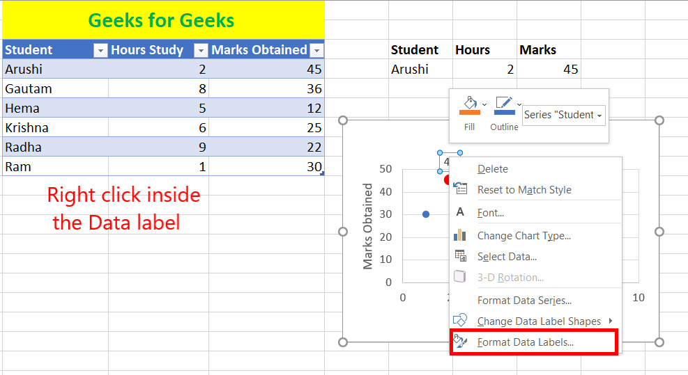
Correlation Chart in Excel - GeeksforGeeks Jun 23, 2021 · The steps to plot a correlation chart are : Select the bivariate data X and Y in the Excel sheet. Go to Insert tab on the top of the Excel window. Select Insert Scatter or Bubble chart. A pop-down menu will appear. Now select the Scatter chart. Now, we need to add a linear trendline in the scatter plot to show the correlation between the ...
Excel Charts - Series Formula
Hiding 0 value data labels in chart - Google Groups the worksheet, make sure you select the chart and take macro>vanishzerolabels>run. Sub VanishZeroLabels () For x = 1 To ActiveChart.SeriesCollection (1).Points.Count If ActiveChart.SeriesCollection...
How to Remove Zero Data Labels in Excel Graph (3 Easy Ways)
Add a Horizontal Line to an Excel Chart - Peltier Tech Verkko11.9.2018 · It should span the chart, starting at X = 0 and ending at X = 6. This is easy, a line simply connects two points, right? We set up a dummy range with our initial and final X and Y values (below, to the left of the top chart), copy the range, select the chart, and use Paste Special to add the data to the chart (see below for details on Paste ...
Excel graph hide data label if = #N/A - Stack Overflow
Change the format of data labels in a chart To get there, after adding your data labels, select the data label to format, and then click Chart Elements > Data Labels > More Options. To go to the appropriate area, click one of the four icons ( Fill & Line, Effects, Size & Properties ( Layout & Properties in Outlook or Word), or Label Options) shown here.
How to hide zero data labels in chart in Excel?
How to Create a Dynamic Chart Range in Excel VerkkoNote that while adding new data automatically updates the chart, deleting data would not completely remove the data points. For example, if you remove 2 data points, the chart will show some empty space on the right. To correct this, drag the blue mark at the bottom right of the Excel table to remove the deleted data points from the table (as ...
Exclude X-Axis Labels If Y-Axis Values Are 0 or Blank in ...
Remove Zero Value Data Labels From Pie Chart - Excel General - OzGrid ... 11,304. Apr 21st 2008. #3. Re: Remove Zero Value Data Labels From Pie Chart. The number format, General;;; would remove zero data labels. Code works for me, so as Dave suggests step through the code. It's possible a value is not truely zero only displayed as such. [h4] Cheers.

Combination Clustered and Stacked Column Chart in Excel ...
How to Quickly Remove Zero Data Labels in Excel - Medium In this article, I will walk through a quick and nifty "hack" in Excel to remove the unwanted labels in your data sets and visualizations without having to click on each one and delete manually....

How to hide zero data labels in chart in Excel?
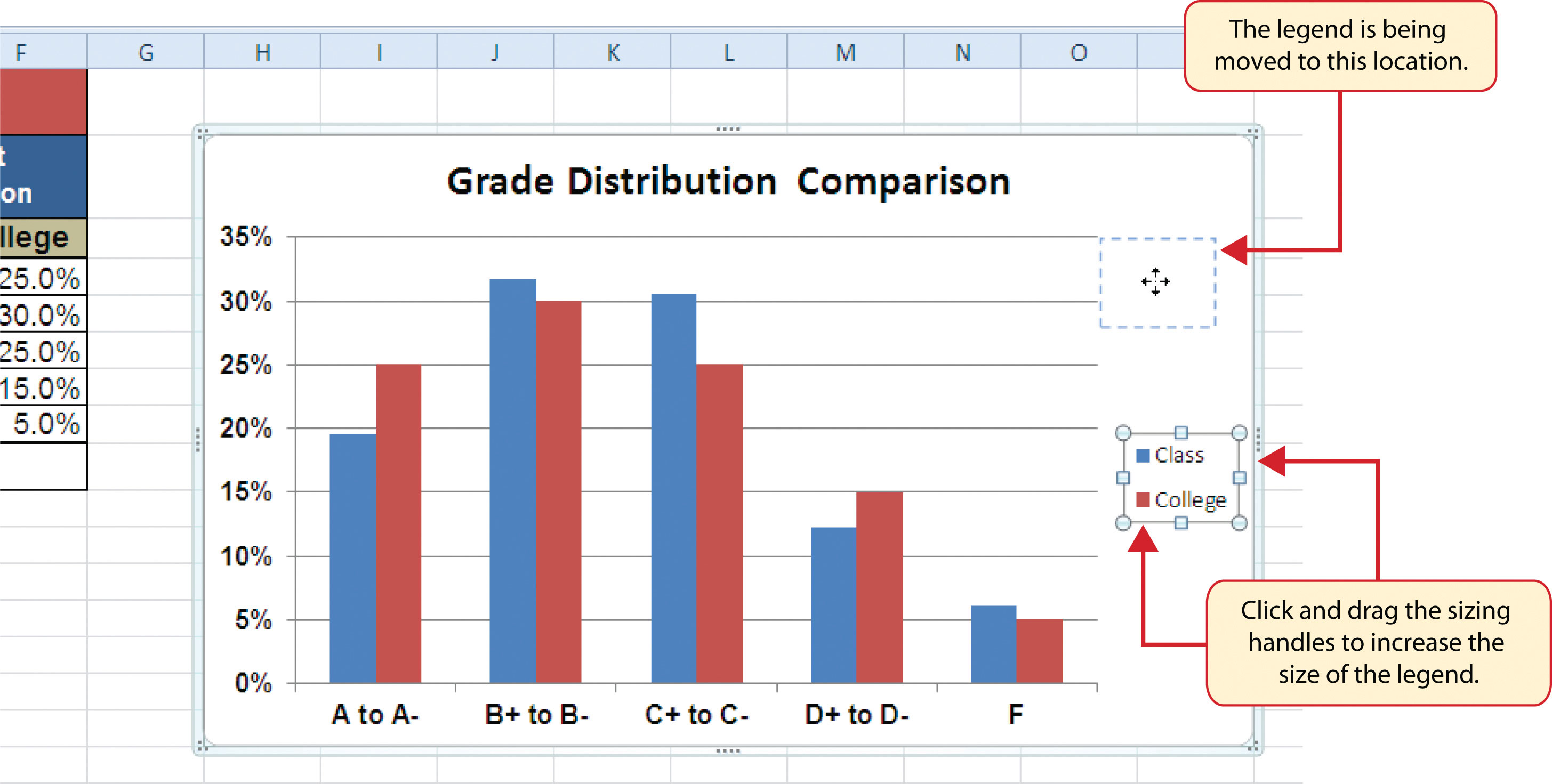
Legends in Chart | How To Add and Remove Legends In Excel Chart… A Legend is a representation of legend keys or entries on the plotted area of a chart or graph, which are linked to the data table of the chart or graph. By default, it may show on the bottom or right side of the chart. The data in a chart is organized with a combination of Series and Categories. Select the chart and choose filter then you will ...
Excel Bar Chart Suppress Zeros
How to rotate axis labels in chart in Excel? - ExtendOffice VerkkoRotate axis labels in Excel 2007/2010. 1. Right click at the axis you want to rotate its labels, select Format Axis from the context menu. See screenshot: 2. In the Format Axis dialog, click Alignment tab and go to the Text Layout section to select the direction you need from the list box of Text direction. See screenshot: 3.

Change the Chart Legend, Data Labels, and Axis Titles : Chart ...
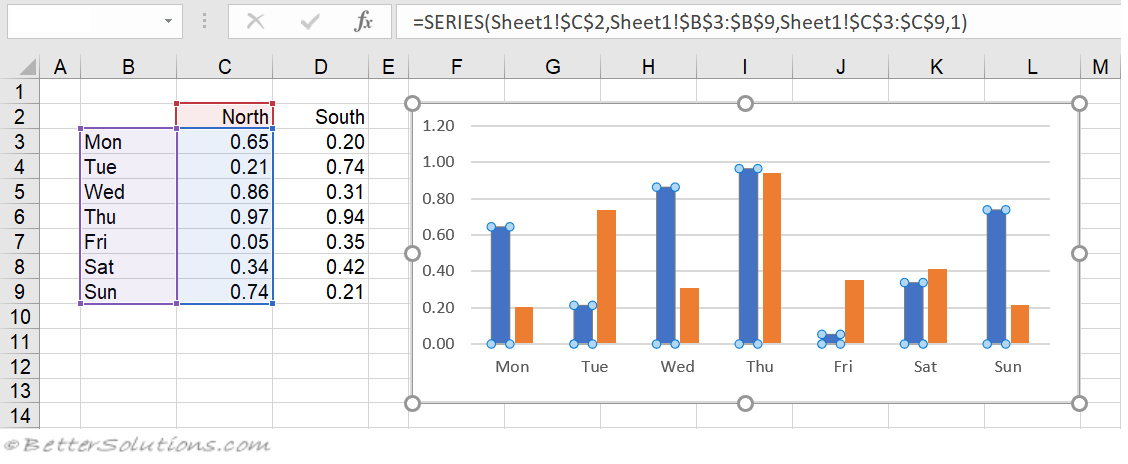
Creating a chart in Excel that ignores #N/A or blank cells VerkkoI am attempting to create a chart with a dynamic data series. Each series in the chart comes from an absolute range, but only a certain amount of that range may have data, and the rest will be #N/A.. The problem is that the chart sticks all of the #N/A cells in as values instead of ignoring them. I have worked around it by using named dynamic …

Apply Custom Data Labels to Charted Points - Peltier Tech

Remove Zero from Chart Data Labels #Shorts

Format Number Options for Chart Data Labels in PowerPoint ...
Set Position of Chart Data Labels in PowerPoint in C#

Show Trend Arrows in Excel Chart Data Labels
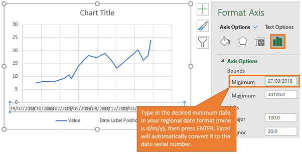
Label Specific Excel Chart Axis Dates • My Online Training Hub
How to remove blank/ zero values from a graph in excel
How to hide zero values in ssrs stacked chart data labels
Formatting Charts
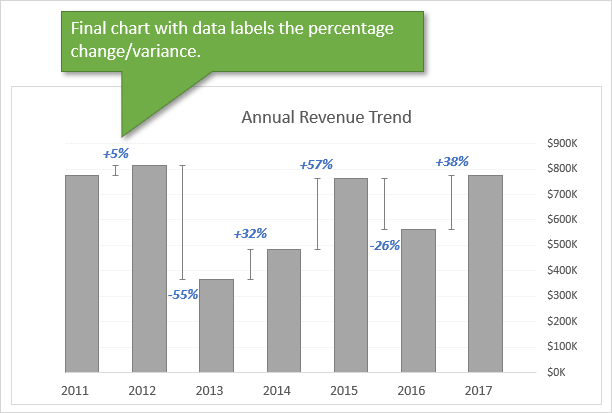
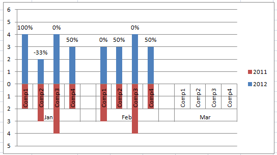
Column Chart That Displays Percentage Change or Variance ...
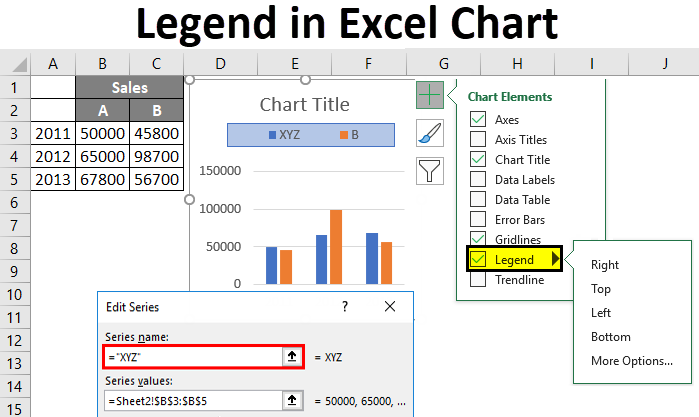
Legends in Chart | How To Add and Remove Legends In Excel Chart?
Hide Series Data Label if Value is Zero - Peltier Tech
How to Find, Highlight, and Label a Data Point in Excel ...

Create a Dynamic Pie Chart with Dynamic Legend in Excel which ...
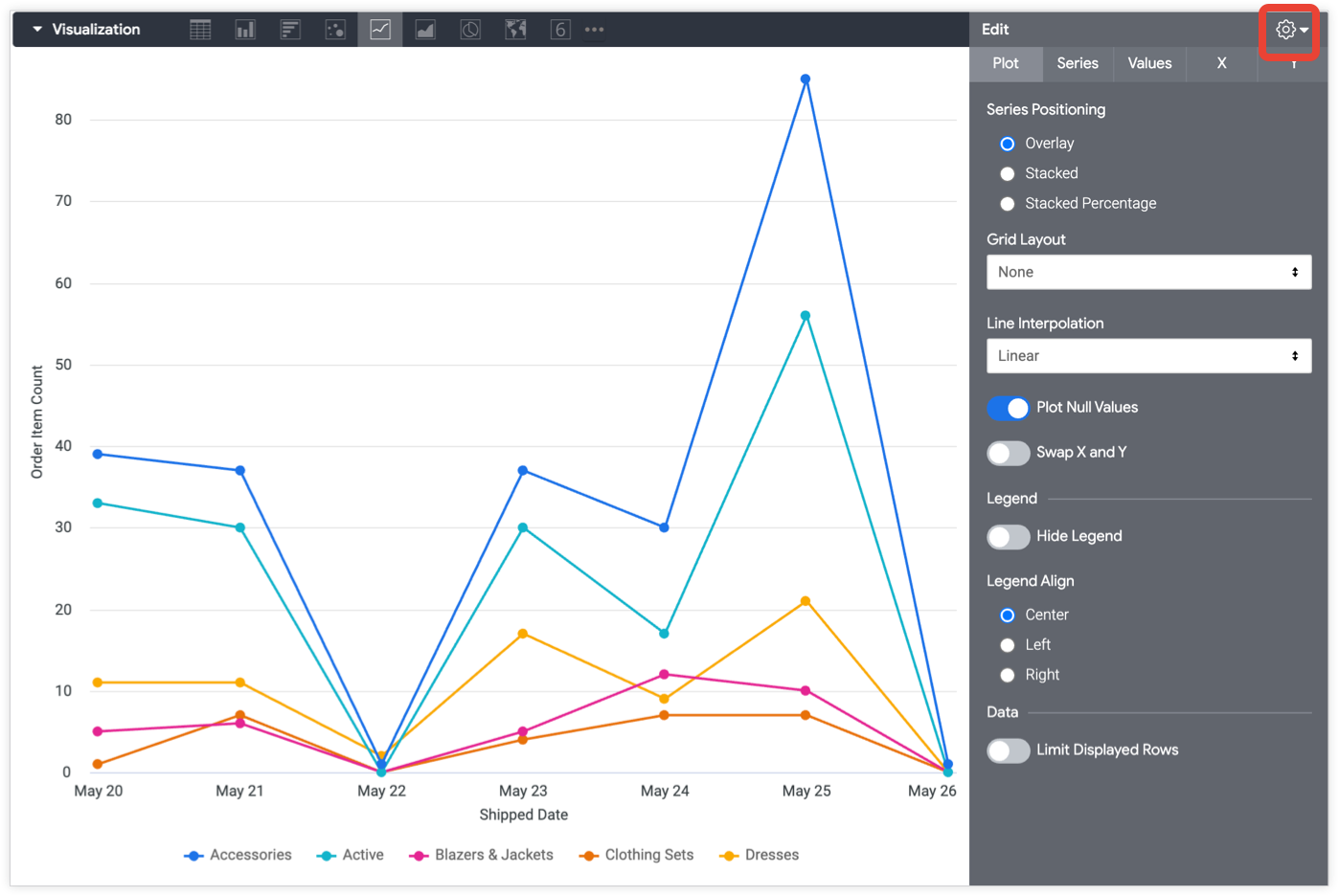
Line chart options | Looker | Google Cloud
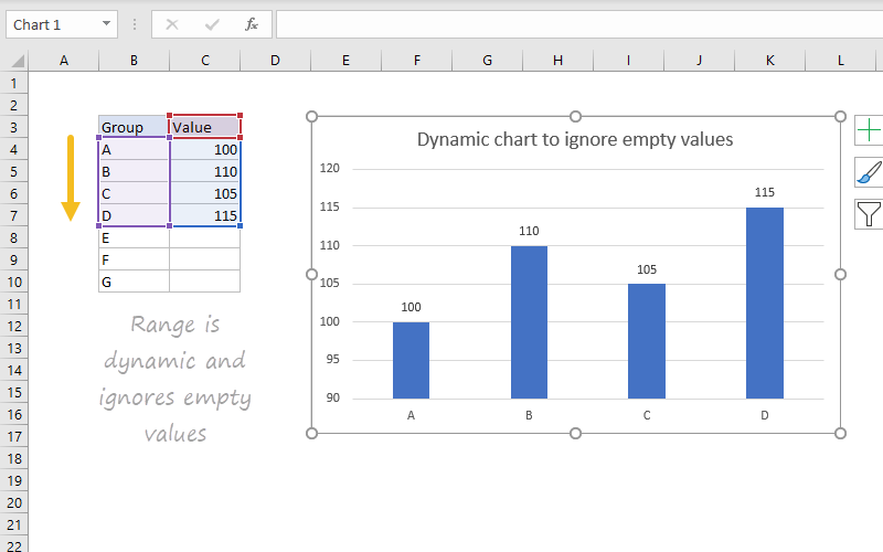
Column chart: Dynamic chart ignore empty values | Exceljet
Add % Difference Data Labels to Excel Horizontal Tornado ...
How to remove a legend label without removing the data series ...
Post a Comment for "40 excel chart remove 0 data labels"