38 data labels excel 2013

How to Create Labels in Word 2013 Using an Excel Sheet How to Create Labels in Word 2013 Using an Excel SheetIn this HowTech written tutorial, we're going to show you how to create labels in Excel and print them ... How to Analyze Data in Excel: Simple Tips and Techniques Ways to Analyze Data in Excel: Tips and Tricks. It is fun to analyze data in MS Excel if you play it right. Here, we offer some quick hacks so that you know how to analyze data in excel. How to Analyze Data in Excel: Data Cleaning; Data Cleaning, one of the very basic excel functions, becomes simpler with a few tips and tricks.

How to Change Excel Chart Data Labels to Custom Values? May 05, 2010 · Now, click on any data label. This will select “all” data labels. Now click once again. At this point excel will select only one data label. Go to Formula bar, press = and point to the cell where the data label for that chart data point is defined. Repeat the process for all other data labels, one after another. See the screencast.

Data labels excel 2013

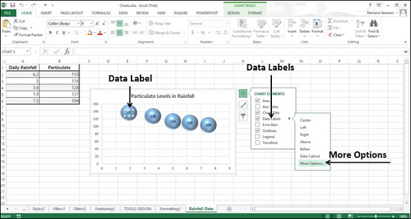
Tip - Adding rich data labels to charts in Excel 2013 You can do this by adjusting the zoom control on the bottom right corner of Excel's chrome. Then, select the value in the data label and hit the right-arrow key on your keyboard. The story behind the data in our example is that the temperature increased significantly on Wednesday and that appeared to help drive up business at the lemonade stand. Custom Axis Labels and Gridlines in an Excel Chart Jul 23, 2013 · Select the vertical dummy series and add data labels, as follows. In Excel 2007-2010, go to the Chart Tools > Layout tab > Data Labels > More Data label Options. In Excel 2013, click the “+” icon to the top right of the chart, click the right arrow next to Data Labels, and choose More Options…. How to insert data labels to a Pie chart in Excel 2013 - YouTube This video will show you the simple steps to insert Data Labels in a pie chart in Microsoft® Excel 2013. Content in this video is provided on an "as is" basis with no express or implied warranties...

Data labels excel 2013. Adding rich data labels to charts in Excel 2013 | Microsoft 365 Blog You can do this by adjusting the zoom control on the bottom right corner of Excel's chrome. Then, select the value in the data label and hit the right-arrow key on your keyboard. The story behind the data in our example is that the temperature increased significantly on Wednesday and that appeared to help drive up business at the lemonade stand. Excel 2013 Tutorial Formatting Data Labels Microsoft Training ... - YouTube FREE Course! Click: about formatting data labels in Microsoft Excel at . A clip from Mastering Excel M... How to Setup Source Data for Pivot Tables - Unpivot in Excel Data Records – Rows in the table below the header that contain the data. Record Set – One row of data that contains values for each field. The data table contains a column for each field and rows for each data record. The column fields are named with descriptive attributes that define the values in the record sets (rows). How to Add Axis Labels in Excel 2013 - YouTube How to Add Axis Labels in Excel 2013For more tips and tricks, be sure to check out is a tutorial on how to add axis labels in E...

Move data labels - support.microsoft.com Right-click the selection > Chart Elements > Data Labels arrow, and select the placement option you want. Different options are available for different chart types. For example, you can place data labels outside of the data points in a pie chart but not in a column chart. Excel Tabular Data • Excel Table • My Online Training Hub Oct 30, 2013 · Note: you could use some complicated formulas to summarise the flat data table into the above report format, but why make your life difficult when you can do it more easily with tabular data. Data Entry Format. The data entry format gets its name due to the intuitive layout which makes it easy for the person keying in the data. Add or remove data labels in a chart - support-uat.microsoft.com Do one of the following: On the Design tab, in the Chart Layouts group, click Add Chart Element, choose Data Labels, and then click None. Click a data label one time to select all data labels in a data series or two times to select just one data label that you want to delete, and then press DELETE. Right-click a data label, and then click ... Tutorial: Import Data into Excel, and Create a Data Model In the next tutorial, Extend Data Model relationships using Excel 2013, Power Pivot, and DAX, you build on what you learned here, and step through extending the Data Model using a powerful and visual Excel add-in called Power Pivot. You also learn how to calculate columns in a table, and use that calculated column so that an otherwise unrelated ...

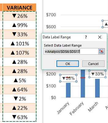
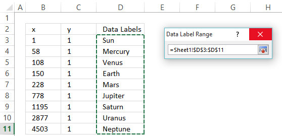
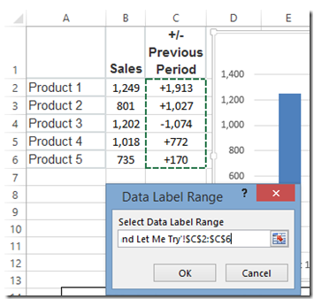
How to Add Data Labels to your Excel Chart in Excel 2013 Data labels show the values next to the corresponding chart element, for instance a percentage next to a piece from a pie chart, or a total value next to a column in a column chart. You can choose... How do I add multiple data labels in Excel? - getperfectanswers Manually add data labels from different column in an Excel chart. Right click the data series in the chart, and select Add Data Labels > Add Data Labels from the context menu to add data labels. Click any data label to select all data labels, and then click the specified data label to select it only in the chart. How To Add Data Labels In Excel - lafacultad.info To add data labels in excel 2013 or excel 2016, follow these steps: To get there, after adding your data labels, select the data label to format, and then click chart elements > data labels > more options. Using Excel Chart Element Button To Add Axis Labels. After That, Select Insert Scatter (X, Y) Or Bubble Chart > Scatter. Add or remove data labels in a chart - support.microsoft.com Right-click the data series or data label to display more data for, and then click Format Data Labels. Click Label Options and under Label Contains, select the Values From Cells checkbox. When the Data Label Range dialog box appears, go back to the spreadsheet and select the range for which you want the cell values to display as data labels.

Quick Tip: Excel 2013 offers flexible data labels | TechRepublic

Excel 2013 Pie Chart Category Data Labels keep Disappearing I have a table in Excel 2013 with 2 slicers - Region and Product Hierarachy, with 5 values in each. I've built a couple pie charts that update when you click on the slicers, to show Market Share by Market Segment. In the pie charts, I formatted the data labels to include Category labels. It works beautifully, until I click one of the slicers.

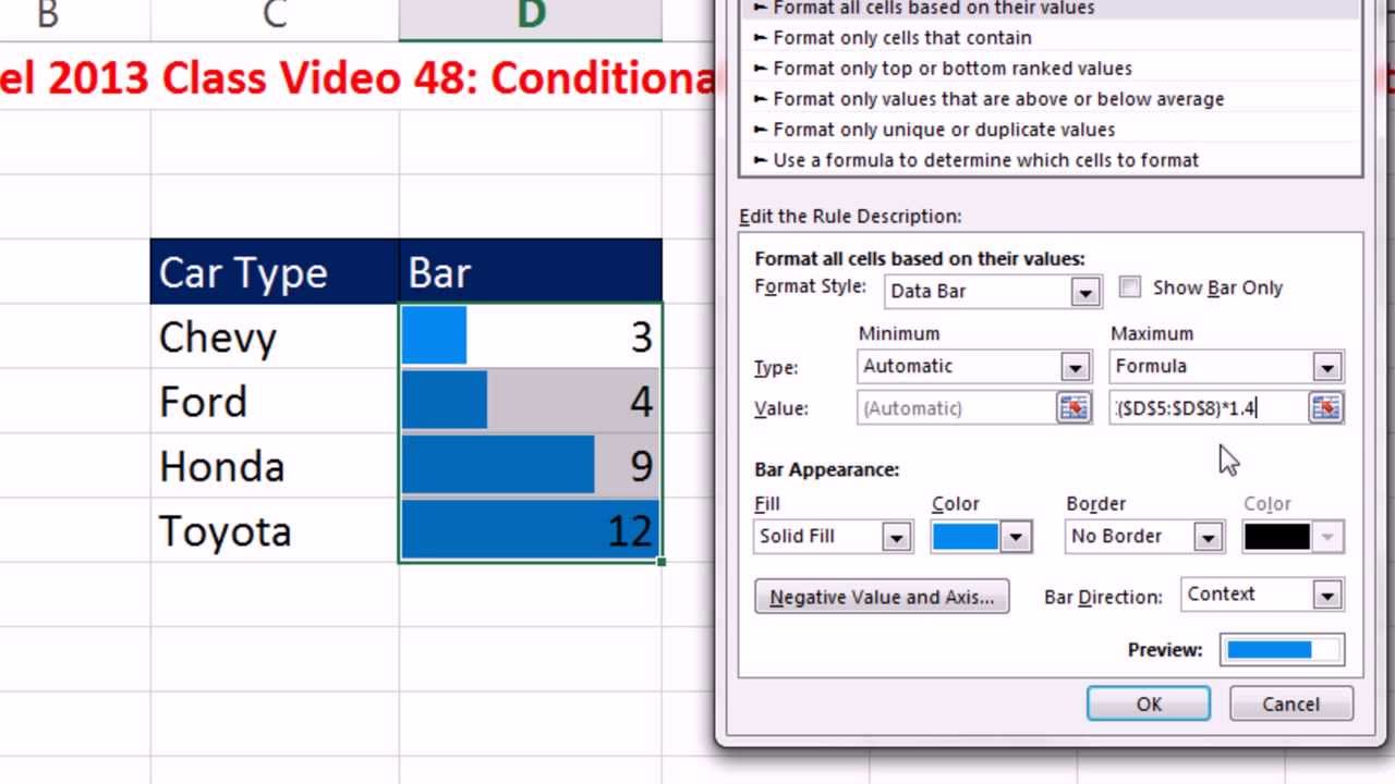
Highline Excel 2013 Class Video 48: Conditional Formatting: Bar Chart with Data Labels

4 steps: How to Create Waterfall Charts in Excel 2013 Select the primary vertical axis (y-axis) and delete as well. Add a chart title -in this case " FY15 Free Cash Flow ". Add data labels by right-clicking one of the series and selecting "Add data labels…". Add labels to each of the series apart from the invisible column. Select the data labels and make them bold, change colour as ...

Custom Data Labels with Colors and Symbols in Excel Charts ...

How to Data Labels in a Line Graph in Excel 2013 - YouTube Want to insert Data Labels in a line graph in Microsoft® Excel 2013? Follow the easy steps shown in this video. Content in this video is provided on an ""as ...

Add or remove data labels in a chart

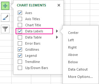
How to Add Data Labels in Excel - Excelchat | Excelchat How to Add Data Labels In Excel 2013 And Later Versions In Excel 2013 and the later versions we need to do the followings; Click anywhere in the chart area to display the Chart Elements button Figure 5. Chart Elements Button Click the Chart Elements button > Select the Data Labels, then click the Arrow to choose the data labels position. Figure 6.

Excel Charts - Aesthetic Data Labels

Quick Tip: Excel 2013 offers flexible data labels | TechRepublic right-click and choose Insert Data Label Field. In the next dialog, select [Cell] Choose Cell. When Excel displays the source dialog, click the cell that contains the MIN () function, and click OK....

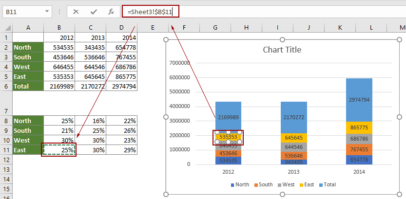
How to show percentages in stacked column chart in Excel?

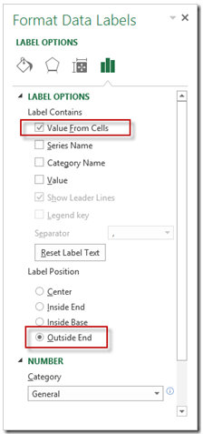
Data Labels in Excel Pivot Chart (Detailed Analysis) Next open Format Data Labels by pressing the More options in the Data Labels. Then on the side panel, click on the Value From Cells. Next, in the dialog box, Select D5:D11, and click OK. Right after clicking OK, you will notice that there are percentage signs showing on top of the columns. 4. Changing Appearance of Pivot Chart Labels

Custom data labels in a chart

data labels in chart - excel 2013 | MrExcel Message Board Hi I have 3 data labels in column chart. I changed the shape of these labels to Oval Callout. if I select one of them to format, then they will be all selected as well. Which is good and understandable. But how can I move them all at same time. Now when I click on one of them then they will all...

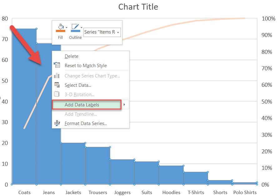
How to Create a Pareto Chart in Excel – Automate Excel

How to Print Labels from Excel - Lifewire Choose Start Mail Merge > Labels . Choose the brand in the Label Vendors box and then choose the product number, which is listed on the label package. You can also select New Label if you want to enter custom label dimensions. Click OK when you are ready to proceed. Connect the Worksheet to the Labels

How to Change Excel Chart Data Labels to Custom Values?

Values From Cell: Missing Data Labels Option in Excel 2013? When a chart created in 2013 using the "Values from Cell" data label option is opened with any earlier version of Excel, the data labels will show as " [CELLRANGE]". If you want to ensure that data labels survive different generations of Excel, you need to revert to the old technique: Insert data labels Edit each individual data label

Custom Chart Labels Using Excel 2013 | MyExcelOnline

How to Add Total Data Labels to the Excel Stacked Bar Chart Apr 03, 2013 · Step 4: Right click your new line chart and select “Add Data Labels” Step 5: Right click your new data labels and format them so that their label position is “Above”; also make the labels bold and increase the font size. Step 6: Right click the line, select “Format Data Series”; in the Line Color menu, select “No line”

Change the format of data labels in a chart

How to insert data labels to a Pie chart in Excel 2013 - YouTube This video will show you the simple steps to insert Data Labels in a pie chart in Microsoft® Excel 2013. Content in this video is provided on an "as is" basis with no express or implied warranties...

Change the format of data labels in a chart

Custom Axis Labels and Gridlines in an Excel Chart Jul 23, 2013 · Select the vertical dummy series and add data labels, as follows. In Excel 2007-2010, go to the Chart Tools > Layout tab > Data Labels > More Data label Options. In Excel 2013, click the “+” icon to the top right of the chart, click the right arrow next to Data Labels, and choose More Options….