39 excel pivot table conditional formatting row labels

Excel tutorial: How to sort a pivot table manually In addition to sorting pivot tables by labels and by values, you can sort a pivot table manually, just by dragging items around. Let’s take a look. Here we have the same pivot table showing sales. Let’s add Product as a Row Label and Region as a Column Label. As you’ve seen previously, both fields are sorted in alphabetical order by default. 101 Advanced Pivot Table Tips And Tricks You Need To Know 25.04.2022 · Without a table your range reference will look something like above. In this example, if we were to add data past Row 51 or Column I our pivot table would not include it in the results. To create and name your table. Select your data. Go to the Insert tab and press the Table button in the Tables section, or use the keyboard shortcut Ctrl + T.

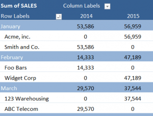
How to remove bold font of pivot table in Excel? - ExtendOffice The normal Bold feature can’t help us to un-bold the row labels in pivot table, but we can apply the powerful function – Conditional Formatting to solve this problem. Please do as follows: 1. Select the bold font row you want to un-bold in the pivot table, or you can press Ctrl key to select multiple bold font rows as your need. See screenshot:

Excel pivot table conditional formatting row labels

How to Group Numbers in Pivot Table in Excel - Trump Excel Sometimes, numbers are stored as text in Excel. In such case, you need to convert these text to numbers before grouping it in Pivot Table. You May Also Like the Following Pivot Table Tutorials: How to Group Dates in Pivot Table in Excel. How to Create a Pivot Table in Excel. Preparing Source Data For Pivot Table. How to Refresh Pivot Table in ... Overwrite pivot table conditional format based on row label Apr 24, 2021 · Hi MRB, As far as I know, using the one rule in the Conditional formatting, we can only format the cells with one color if the condition is true and if the same condition is false, the formatting of the cell will be blank and if both conditions are true, the formatting of cell depends on the highest ranking/priority of the rules in Conditional formatting. How to Insert a Blank Row in Excel Pivot Table | MyExcelOnline 17.01.2021 · Pivot Table reports are shown in a Compact Layout format as a default and if you have two or more Items in the Row Labels (e.g.Month & Customer), then the Pivot Table report can look very clunky…. There is a cool little trick that most Excel users do not know about that adds a blank row after each item, making the Pivot Table report look more appealing.

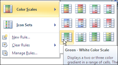
Excel pivot table conditional formatting row labels. How to Apply Conditional Formatting in Pivot Table? (with ... Easy Steps to Apply Conditional Formatting in the Pivot Table. First, we must select the data. Then, in the “Insert” Tab, click on “Pivot Tables.”. As a result, a dialog box appears. Next, we must insert the pivot table in a new worksheet by clicking “OK.”. Currently, a pivot table is blank. Next, ... EXCEL: SETTING PIVOT TABLE DEFAULTS - Strategic Finance 01.04.2017 · The second way to set the defaults is useful if you have a pivot table that’s already in the correct format. You can base the defaults on that pivot table. Open the workbook that contains the pivot table. Select one cell in the pivot table. Go to File, Options, Advanced, Data, and click the button for Edit Default Layout. How to Replace Blank Cells with Zeros in Excel Pivot Tables In Pivot Table Options Dialogue Box, within the Layout & Format tab, make sure that the For Empty cells show option is checked, and enter 0 in the field next to it. If you want to can replace blank cells with text such as NA or No Sales. Click OK. That’s it! Now all the blank cells would automatically show 0. You can also play around with the ... Excel Conditional Formatting in Pivot Table - EDUCBA Go to the HOME tab > Click on Conditional Formatting option under Styles > Click on Highlight Cells Rules option > Click on Less Than option. It will open a Less Than dialog box. Enter 1500 under the Format Cells field and choose a color as “Yellow Fill with Dark Yellow Text”. Refer to the below screenshot. And then click on OK.

How to Apply Conditional Formatting to Pivot Tables - Excel ... Dec 13, 2018 · How to Setup Conditional Formatting for Pivot Tables. 1. Select a cell in the Values area. The first step is to select a cell in the Values area of the pivot table. If your pivot table has multiple fields ... 2. Apply Conditional Formatting. 3. Using the Formatting Options Menu. 4. Accessing the ... The Pivot table tools ribbon in Excel These two tabs allow you to perform pivot table customization. This is the Pivot table ribbon in Excel. Create pivot table fields , charts and sets. Here is an important thing to wonder for the pivot table ribbon in excel is as soon as you switch the selected cell to non pivot table cell. The pivot table ribbon disappears. So it means Excel ... 101 Excel Pivot Tables Examples | MyExcelOnline 31.07.2020 · Pivot Tables in Excel are one of the most powerful features within Microsoft Excel. An Excel Pivot Table allows you to analyze more than 1 million rows of data with just a few mouse clicks, show the results in an easy to read table, “pivot”/change the report layout with the ease of dragging fields around, highlight key information to management and include Charts & … How to Apply Conditional Formatting to Pivot Tables - Excel … 13.12.2018 · Bottom Line: Learn how to apply conditional formatting to pivot tables so that the formats are dynamically reapplied as the pivot table is changed, filtered, or updated. Skill Level: Intermediate Download the Excel File. Here's the file that I use in the video. You can use it to practice adding, deleting, and changing conditional formatting on a variety of pivot table …

How to Insert a Blank Row in Excel Pivot Table | MyExcelOnline 17.01.2021 · Pivot Table reports are shown in a Compact Layout format as a default and if you have two or more Items in the Row Labels (e.g.Month & Customer), then the Pivot Table report can look very clunky…. There is a cool little trick that most Excel users do not know about that adds a blank row after each item, making the Pivot Table report look more appealing. Overwrite pivot table conditional format based on row label Apr 24, 2021 · Hi MRB, As far as I know, using the one rule in the Conditional formatting, we can only format the cells with one color if the condition is true and if the same condition is false, the formatting of the cell will be blank and if both conditions are true, the formatting of cell depends on the highest ranking/priority of the rules in Conditional formatting. How to Group Numbers in Pivot Table in Excel - Trump Excel Sometimes, numbers are stored as text in Excel. In such case, you need to convert these text to numbers before grouping it in Pivot Table. You May Also Like the Following Pivot Table Tutorials: How to Group Dates in Pivot Table in Excel. How to Create a Pivot Table in Excel. Preparing Source Data For Pivot Table. How to Refresh Pivot Table in ...

Excel Spreadsheets Help: How to Make Alternating Row Colors in Excel

How to Insert a Blank Row in Excel Pivot Table | MyExcelOnline