45 how to add data labels to a 3d pie chart in excel
How to Create Pie Charts in Excel: The Ultimate Guide How to Add Labels to a Pie Chart in Excel. Adding labels to a pie chart is a great way to provide additional information about the data in the chart. To add click format data labels, select the pie chart and then go to the ribbon and click on the Add Data Labels button. This will add data labels for each pie chart slice that show the value of ... adding decimal places to percentages in pie charts Hello DV_1956. I am V. Arya, Independent Advisor, to work with you on this issue. Right click on your % label - Format Data labels. Beneath Number choose percentage as category. Report abuse. 44 people found this reply helpful. ·. Was this reply helpful?
How to show data labels in charts created via Openpyxl 2 Answers. This works for me on a line chart (As a combination chart): openpyxls version: 2.3.2: from openpyxl.chart.label import DataLabelList chart2 = LineChart () .... code to build chart like add_data () and: # Style the lines s1 = chart2.series [0] s1.marker.symbol = "diamond" ... your data labels added here: chart2.dataLabels ...
How to add data labels to a 3d pie chart in excel
EOF How to add data labels from different column in an Excel chart? Click any data label to select all data labels, and then click the specified data label to select it only in the chart. 3. Go to the formula bar, type =, select the corresponding cell in the different column, and press the Enter key. See screenshot: 4. Repeat the above 2 - 3 steps to add data labels from the different column for other data points. Creating Pie Chart and Adding/Formatting Data Labels (Excel) Creating Pie Chart and Adding/Formatting Data Labels (Excel) Creating Pie Chart and Adding/Formatting Data Labels (Excel)
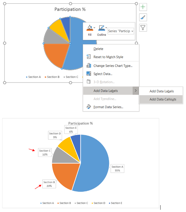
How to add data labels to a 3d pie chart in excel. Edit titles or data labels in a chart - support.microsoft.com On a chart, click one time or two times on the data label that you want to link to a corresponding worksheet cell. The first click selects the data labels for the whole data series, and the second click selects the individual data label. Right-click the data label, and then click Format Data Label or Format Data Labels. How to Create a 3D Pie Chart in Excel (with Easy Steps) As a result, it will add the Data Labels to your 3D pie chart. Now, in order to format the Data Labels, click on any Data Label and right-click on your mouse. Hence, a pop-up window will appear. After that, click on the Format Data Labels option from the pop-up window. How to Make a Pie Chart in Excel & Add Rich Data Labels to The Chart! 7) With the data point still selected, go to Chart Tools>Format>Shape Styles and click on the drop-down arrow next to Shape Effects and select Shadow and choose Inner Shadow>Inside Diagonal Top Left. 8) With the one data point still selected, right-click this data point, and select Add Data Label>Add Data Callout as shown below. Excel 3-D Pie charts - Microsoft Excel 2016 - OfficeToolTips If you want to create a pie chart that shows your company (in this example - Company A) in the greatest positive light: Do the following: 1. Select the data range (in this example, B5:C10 ). 2. On the Insert tab, in the Charts group, choose the Pie button: Choose 3-D Pie. 3. Right-click in the chart area, then select Add Data Labels and click ...
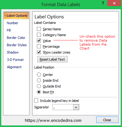
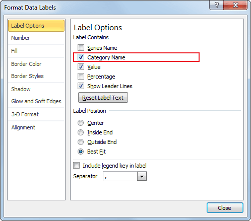
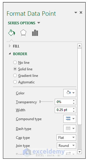
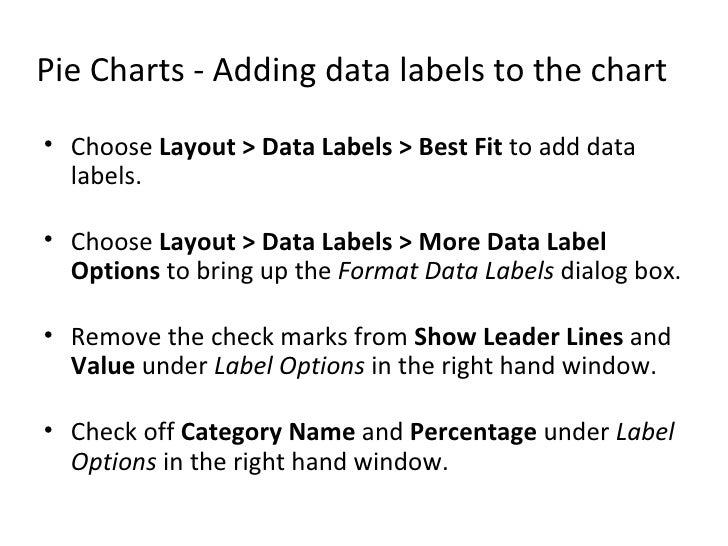
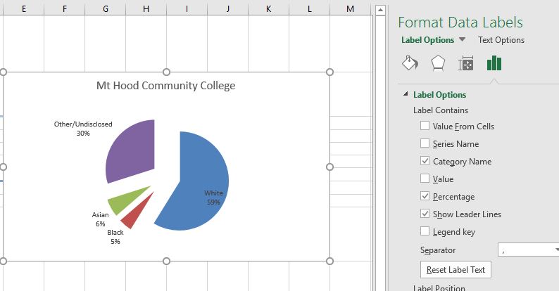
How to insert data labels to a Pie chart in Excel 2013 - YouTube This video will show you the simple steps to insert Data Labels in a pie chart in Microsoft® Excel 2013. Content in this video is provided on an "as is" basi... How to display leader lines in pie chart in Excel? - ExtendOffice To display leader lines in pie chart, you just need to check an option then drag the labels out. 1. Click at the chart, and right click to select Format Data Labels from context menu. 2. In the popping Format Data Labels dialog/pane, check Show Leader Lines in the Label Options section. See screenshot: 3. How to ☝️Create A 3-D Pie Chart in Excel - SpreadsheetDaddy Right-click on your 3-D pie graph and click " Add Data Labels. " Go to the Label Options tab. Check the " Category Name " box to display the names of the categories along with the actual market share data. Recolor the Slices Next stop: changing the color of the slices.Double-click on the slice you want to recolor and select " Format Data Point. " Add or remove data labels in a chart - support.microsoft.com Click the data series or chart. To label one data point, after clicking the series, click that data point. In the upper right corner, next to the chart, click Add Chart Element > Data Labels. To change the location, click the arrow, and choose an option. If you want to show your data label inside a text bubble shape, click Data Callout.
How to Create and Format a Pie Chart in Excel - Lifewire To add data labels to a pie chart: Select the plot area of the pie chart. Right-click the chart. Select Add Data Labels . Select Add Data Labels. In this example, the sales for each cookie is added to the slices of the pie chart. Change Colors Pie Chart in Excel | How to Create Pie Chart - EDUCBA Step 1: Select the data to go to Insert, click on PIE, and select 3-D pie chart. Step 2: Now, it instantly creates the 3-D pie chart for you. Step 3: Right-click on the pie and select Add Data Labels. This will add all the values we are showing on the slices of the pie. Display data point labels outside a pie chart in a paginated report ... To display data point labels inside a pie chart. Add a pie chart to your report. For more information, see Add a Chart to a Report ... On the 3D Options tab, select Enable 3D. If you want the chart to have more room for labels but still appear two-dimensional, set the Rotation and Inclination properties to 0. See Also. Creating Pie Chart and Adding/Formatting Data Labels (Excel) Creating Pie Chart and Adding/Formatting Data Labels (Excel) Creating Pie Chart and Adding/Formatting Data Labels (Excel)
How to Create a Pie Chart in Excel using Worksheet Data
How to add data labels from different column in an Excel chart? Click any data label to select all data labels, and then click the specified data label to select it only in the chart. 3. Go to the formula bar, type =, select the corresponding cell in the different column, and press the Enter key. See screenshot: 4. Repeat the above 2 - 3 steps to add data labels from the different column for other data points.
Excel 3-D Pie charts - Microsoft Excel 2010
EOF

Microsoft Excel Tutorials: Add Data Labels to a Pie Chart

Rotate Pie Chart in Excel | How to Rotate Pie Chart in Excel?
How to Make a Pie Chart in Word 2010 | Doovi
How to Make a Pie Chart in Excel & Add Rich Data Labels to The Chart!
How to Create Excel Pie Charts & Add Rich Data Labels to The Chart!
Charts in excel 2007
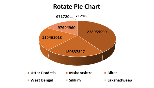
Rotate Pie Chart in Excel | How to Rotate Pie Chart in Excel?

Excel 3-D Pie charts - Microsoft Excel 2016
Pie Chart Techniques | Experts Exchange
4.1 Choosing a Chart Type – Excel For Decision Making
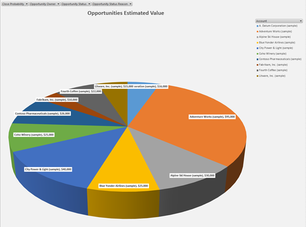
Power BI Microsoft Dynamics CRM Online – PivotChart Report Part 2 | Magnetism Solutions | NZ ...

How to Create a Pie Chart in Excel | Smartsheet

microsoft excel - How to make a Pie radar chart - Super User
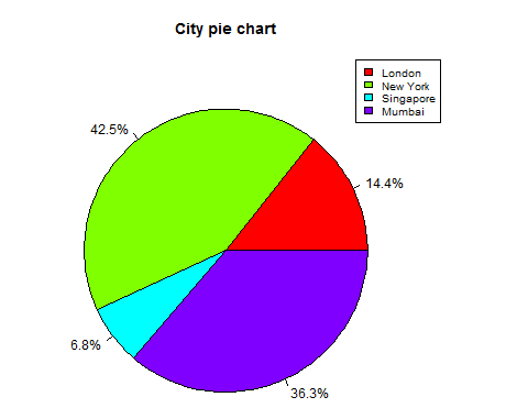
R - Pie Charts
ExcelSirJi | Excel Data Tips | How to Create Pie Chart in Excel (Complete Tutorial) ExcelSirJi
How to Make a Pie Chart in Excel & Add Rich Data Labels to The Chart!
Post a Comment for "45 how to add data labels to a 3d pie chart in excel"