43 conditional formatting data labels excel

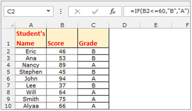
Excel Data Analysis - Conditional Formatting Follow the steps to conditionally format cells − Select the range to be conditionally formatted. Click Conditional Formatting in the Styles group under Home tab. Click Highlight Cells Rules from the drop-down menu. Click Greater Than and specify >750. Choose green color. Click Less Than and specify < 500. Choose red color. How to Use Conditional Formatting Based on Date in Microsoft Excel Open the sheet, select the cells you want to format, and head to the Home tab. In the Styles section of the ribbon, click the drop-down arrow for Conditional Formatting. Move your cursor to Highlight Cell Rules and choose "A Date Occurring" in the pop-out menu. A small window appears for you to set up your rule.

How to do conditional formatting of a label in Excel VBA Function ConditionalFormatNumber (n As Double) As String If n > 1000000 Then ConditionalFormatNumber = Format (n / 1000000, "$#,##0.00,,""M""") ElseIf n > 1000 Then ConditionalFormatNumber = Format (n / 1000, "$#,##0.00, ""K""") Else ConditionalFormatNumber = Format (n, "$#,##0.0") End If End Function Share Improve this answer

Conditional formatting data labels excel

Custom Data Labels with Colors and Symbols in Excel Charts - [How To] Step 4: Select the data in column C and hit Ctrl+1 to invoke format cell dialogue box. From left click custom and have your cursor in the type field and follow these steps: Press and Hold ALT key on the keyboard and on the Numpad hit 3 and 0 keys. Let go the ALT key and you will see that upward arrow is inserted. How to Create Excel Charts (Column or Bar) with Conditional Formatting Conditional formatting is the practice of assigning custom formatting to Excel cells—color, font, etc.—based on the specified criteria (conditions). The feature helps in analyzing data, finding statistically significant values, and identifying patterns within a given dataset. Conditional Formatting Shapes - Step by step Tutorial Let's see step by step how to create it: First, select an already formatted cell. In the picture below, we have created a little example of this. We will pay attention to the range D5:D6. You can see the rules in the Rules Manager window. We didn't make it overly complicated.

Conditional formatting data labels excel. How to add conditional colouring to Scatterplots in Excel Step 3: Edit the colours. To edit the colours, select the chart -> Format -> Select Series A from the drop down on top left. In the format pane, select the fill and border colours for the marker. Repeat these steps for Series B and Series C. Here is our final scatterplot. Change the format of data labels in a chart To get there, after adding your data labels, select the data label to format, and then click Chart Elements > Data Labels > More Options. To go to the appropriate area, click one of the four icons ( Fill & Line, Effects, Size & Properties ( Layout & Properties in Outlook or Word), or Label Options) shown here. Changing the Color of a Data Label using IF Statement 1) Click on the data labels to highlight all the data labels, 2) Right-Click and select Format Data Labels, 3) Click on Number, 4) Go to the Format Code field *adapt the following to your needs* 5) [green] [>29]#.00; [<30] [Color 53]#.00 Click to expand... Hi Jawnne, I hope you're still lurking about on here. Conditional Formatting with Data Validation - Microsoft Tech Community For example, if A2=Value, B2= Value, and C2 is blank, I would like to have C2 turn red. A2,B2, and C2 all have a list range for the Data Validation. For the conditional formatting, I have only put the range to apply to as column C. The conditional formatting is not turning cells red as needed. I am not sure what the issue is.

Format Data Labels in Excel- Instructions - TeachUcomp, Inc. One way to do this is to click the "Format" tab within the "Chart Tools" contextual tab in the Ribbon. Then select the data labels to format from the "Current Selection" button group. Then click the "Format Selection" button that appears below the drop-down menu in the same area. Conditional format chart data labels | Dashboards & Charts | Excel ... Lance 354 524 550 I create a bar chart that from this data, and display the data label for Actual. I would like to format this data label so that it displays in Red if the value of Actual is less than the value of On Track. Otherwise, it will just display as Blue, which is the format color right now. Excel tutorial: How to use data labels Generally, the easiest way to show data labels to use the chart elements menu. When you check the box, you'll see data labels appear in the chart. If you have more than one data series, you can select a series first, then turn on data labels for that series only. You can even select a single bar, and show just one data label. Custom Chart Data Labels In Excel With Formulas Follow the steps below to create the custom data labels. Select the chart label you want to change. In the formula-bar hit = (equals), select the cell reference containing your chart label's data. In this case, the first label is in cell E2. Finally, repeat for all your chart laebls.

Conditional formatting chart data labels? - Excel Help Forum The easy way to conditionally format these labels is use two series. Use something like =IF ($E2=1,0,NA ()) for the series that has red labels and =IF (#E2=1,NA (),0) for the series that has unformatted labels. Jon Peltier Register To Reply Similar Threads Conditional Number Formatting Not Working for Chart Value Labels Excel tutorial: How to add a conditional formatting key That way, we can adjust the conditions for the rules using the key itself. The first step is to create the basic layout for the key. For this, we'll set up a small table with three rows - one for each conditional format. We can then add labels for each conditional format rule. These could be anything, but let's use Excellent, Concern, and ... Conditional formatting - Microsoft Tech Community You can try this rule for conditional formatting. In your initial question and example it seems that you only want to highlight the value of the first non-empty cell of column T. Only this value is highlighted in column P in your example. 0 Likes Reply Excel Conditional Formatting - Data Bars - W3Schools Click on the Conditional Formatting icon in the ribbon, from Home menu. Select Data Bars from the drop-down menu. Select the "Green Data Bars" color option from the Gradient Fill menu. Note: Both Gradient Fill and Solid Fill work the same way. The only difference between those, and the color options are aesthetic.

How to Create Multi-Category Chart in Excel - Excel Board

VBA Conditional Formatting of Charts by Value and Label The category labels (XValues) and values (Values) are put into arrays, also for ease of processing. The code then looks at each point's value and label, to determine which cell has the desired formatting. The rows and columns are looped starting at 2, since the first of each contains an irrelevant label. The looping stops one count before the end.

How to Create Multi-Category Chart in Excel - Excel Board

Conditional Formatting in Excel (In Easy Steps) 1. Select the range A1:A10. 2. On the Home tab, in the Styles group, click Conditional Formatting. 3. Click Highlight Cells Rules, Greater Than. 4. Enter the value 80 and select a formatting style. 5. Click OK. Result. Excel highlights the cells that are greater than 80. 6. Change the value of cell A1 to 81. Result.

How To Use Conditional Formatting in Excel - YouTube

How to create a chart with conditional formatting in Excel? Add three columns right to the source data as below screenshot shown: (1) Name the first column as >90, type the formula =IF (B2>90,B2,0) in the first blank cell of this column, and then drag the AutoFill Handle to the whole column;

HIGHLIGHT DUPLICATE VALUE IN EXCEL - Data analysis

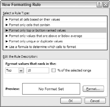
How to Apply Conditional Formatting to Rows Based on ... - Excel Campus On the Home tab of the Ribbon, select the Conditional Formatting drop-down and click on Manage Rules…. That will bring up the Conditional Formatting Rules Manager window. Click on New Rule. This will open the New Formatting Rule window. Under Select a Rule Type, choose Use a formula to determine which cells to format.

How to use Conditional Formatting in Excel? - GeeksforGeeks

How to change chart axis labels' font color and size in Excel? Sometimes, you may want to change labels' font color by positive/negative/ in an axis in chart. You can get it done with conditional formatting easily as follows: 1. Right click the axis you will change labels by positive/negative/0, and select the Format Axis from right-clicking menu. 2.

Chapter 19: Conditional Formatting and Data Validation | Excel 2007 Formulas (Mr. Spreadsheets ...

Excel conditional formatting Icon Sets, Data Bars and Color Scales Select all cells in column A, except for the column header, and create a conditional formatting icon set rule by clicking Conditional Formatting > Icon sets > More Rules... In the New Formatting Rule dialog, select the following options: Click the Reverse Icon Order button to change the icons' order. Select the Icon Set Only checkbox.

How to Create a MS Excel Pivot Table – An Introduction | SIMPLE TAX INDIA

Conditional formatting for Excel column charts - Think Outside The Slide Additional formatting. The colors used for each data series is from the color theme being used for this Excel file. You can assign more meaningful colors for each data series. You can also add data labels to each series. It is a good idea to format the data label text to have the same color as the column it is representing.

excel - Save applied formats of conditional formatting - Stack Overflow

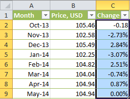
Use conditional formatting to highlight information Conditional formatting can help make patterns and trends in your data more apparent. To use it, you create rules that determine the format of cells based on their values, such as the following monthly temperature data with cell colors tied to cell values.

Conditional Formatting in Excel - The Ultimate Guide

Conditional Formatting in Excel - a Beginner's Guide Click Conditional Formatting, then select Icon Set to choose from various shapes to help label your data. For this example, let's use the arrow icon set to show whether our highlighted data, the Variance column, has increased or decreased. Now, you'll see that the data has arrow icons accompanying their values in the cells.

Advanced Graphs Using Excel : Heat map plot in excel using conditional formatting

Conditional Formatting Shapes - Step by step Tutorial Let's see step by step how to create it: First, select an already formatted cell. In the picture below, we have created a little example of this. We will pay attention to the range D5:D6. You can see the rules in the Rules Manager window. We didn't make it overly complicated.

How to Create Multi-Category Chart in Excel - Excel Board

How to Create Excel Charts (Column or Bar) with Conditional Formatting Conditional formatting is the practice of assigning custom formatting to Excel cells—color, font, etc.—based on the specified criteria (conditions). The feature helps in analyzing data, finding statistically significant values, and identifying patterns within a given dataset.