39 add data labels to excel chart

Add Custom Labels to x-y Scatter plot in Excel Step 1: Select the Data, INSERT -> Recommended Charts -> Scatter chart (3 rd chart will be scatter chart) Let the plotted scatter chart be. Step 2: Click the + symbol and add data labels by clicking it as shown below. Step 3: Now we need to add the flavor names to the label. Now right click on the label and click format data labels. Edit titles or data labels in a chart - support.microsoft.com On a chart, click one time or two times on the data label that you want to link to a corresponding worksheet cell. The first click selects the data labels for the whole data series, and the second click selects the individual data label. Right-click the data label, and then click Format Data Label or Format Data Labels.

Add data labels and callouts to charts in Excel 365 | EasyTweaks.com The steps that I will share in this guide apply to Excel 2021 / 2019 / 2016. Step #1: After generating the chart in Excel, right-click anywhere within the chart and select Add labels . Note that you can also select the very handy option of Adding data Callouts.

Add data labels to excel chart

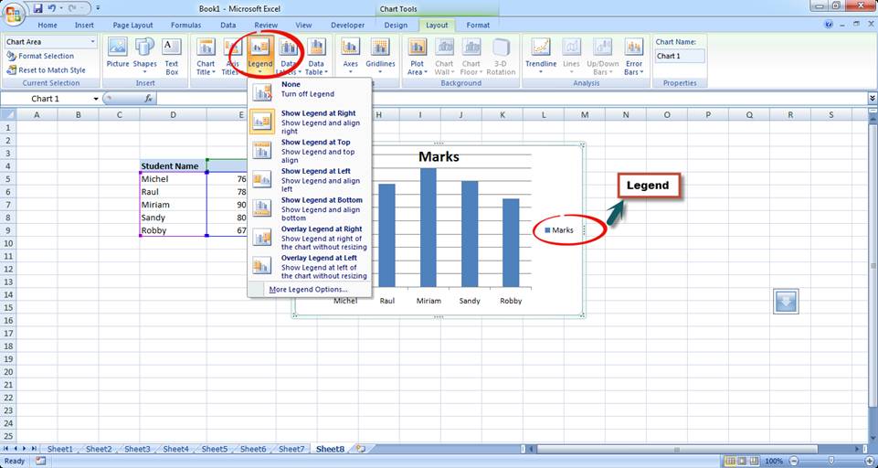
Add / Move Data Labels in Charts - Excel & Google Sheets Adding Data Labels Click on the graph Select + Sign in the top right of the graph Check Data Labels Change Position of Data Labels Click on the arrow next to Data Labels to change the position of where the labels are in relation to the bar chart Final Graph with Data Labels How to Add Data Labels in Excel - Excelchat | Excelchat After inserting a chart in Excel 2010 and earlier versions we need to do the followings to add data labels to the chart; Click inside the chart area to display the Chart Tools. Figure 2. Chart Tools Click on Layout tab of the Chart Tools. In Labels group, click on Data Labels and select the position to add labels to the chart. Figure 3. Use a screen reader to add a title, data labels, and a legend to a ... Select the chart that you want to work with. To open the Add Chart Element menu, press Alt+J, C, A. Select the type of title you want to add: To add a chart title, press C. The focus moves to the Chart title list. Do one of the following: To add a title above the chart, press A, type a title, and then press Enter.

Add data labels to excel chart. Select Data to Display in an Excel Chart With Option Buttons Feb 17, 2015 · When the formulas don’t show the values, they will not appear in the chart. The Data. The extended data range is shown below. At first the formula in cell F2 (and copied into the entire range F2:I13) is simply =B2. To give the user a choice, add two option buttons and label them Chart A and Chart B. Add vertical line to Excel chart: scatter plot, bar and line ... May 15, 2019 · Insert vertical line in Excel bar chart; Add vertical line to line chart; How to add vertical line to scatter plot. To highlight an important data point in a scatter chart and clearly define its position on the x-axis (or both x and y axes), you can create a vertical line for that specific data point like shown below: How to add data labels from different column in an Excel chart? This method will introduce a solution to add all data labels from a different column in an Excel chart at the same time. Please do as follows: 1. Right click the data series in the chart, and select Add Data Labels > Add Data Labels from the context menu to add data labels. 2. Add or remove data labels in a chart - support.microsoft.com Depending on what you want to highlight on a chart, you can add labels to one series, all the series (the whole chart), or one data point. Add data labels. You can add data labels to show the data point values from the Excel sheet in the chart. This step applies to Word for Mac only: On the View menu, click Print Layout.

Change the format of data labels in a chart To get there, after adding your data labels, select the data label to format, and then click Chart Elements > Data Labels > More Options. To go to the appropriate area, click one of the four icons ( Fill & Line, Effects, Size & Properties ( Layout & Properties in Outlook or Word), or Label Options) shown here. Custom Chart Data Labels In Excel With Formulas Follow the steps below to create the custom data labels. Select the chart label you want to change. In the formula-bar hit = (equals), select the cell reference containing your chart label's data. In this case, the first label is in cell E2. Finally, repeat for all your chart laebls. How to Customize Your Excel Pivot Chart Data Labels - dummies The Data Labels command on the Design tab's Add Chart Element menu in Excel allows you to label data markers with values from your pivot table. When you click the command button, Excel displays a menu with commands corresponding to locations for the data labels: None, Center, Left, Right, Above, and Below. None signifies that no data labels should be added to the chart and Show signifies ... How to add total labels to stacked column chart in Excel? Select and right click the new line chart and choose Add Data Labels > Add Data Labels from the right-clicking menu. See screenshot: And now each label has been added to corresponding data point of the Total data series. And the data labels stay at upper-right corners of each column. 5.

How to add axis label to chart in Excel? - ExtendOffice 1. Select the chart that you want to add axis label. 2. Navigate to Chart Tools Layout tab, and then click Axis Titles, see screenshot: 3. You can insert the horizontal axis label by clicking Primary Horizontal Axis Title under the Axis Title drop down, then click Title Below Axis, and a text box will appear at the bottom of the chart, then you ... Adding rich data labels to charts in Excel 2013 - Microsoft 365 Blog To add a data label in a shape, select the data point of interest, then right-click it to pull up the context menu. Click Add Data Label, then click Add Data Callout . The result is that your data label will appear in a graphical callout. In this case, the category Thr for the particular data label is automatically added to the callout too. Adding Data Labels To An Excel Chart | MyExcelOnline In our example below, I add a Data Label to a column chart and then I format the data label using CTRL+1. I then select to custom format the numbers so it shows the values as thousands by adding a comma , after each zero and then showing the work k by adding "k" Example Custom Number Format: [$$-1004]#,##0 ,"k" ;- [$$-1004]#,##0 ,"k" Excel charts: add title, customize chart axis, legend and data labels ... Click the Chart Elements button, and select the Data Labels option. For example, this is how we can add labels to one of the data series in our Excel chart: For specific chart types, such as pie chart, you can also choose the labels location. For this, click the arrow next to Data Labels, and choose the option you want.

How to Add Data Labels in Excel - Excelchat | Excelchat

How to create Custom Data Labels in Excel Charts Create the chart as usual. Add default data labels. Click on each unwanted label (using slow double click) and delete it. Select each item where you want the custom label one at a time. Press F2 to move focus to the Formula editing box. Type the equal to sign. Now click on the cell which contains the appropriate label.

Multiple Series in One Excel Chart - Peltier Tech Blog

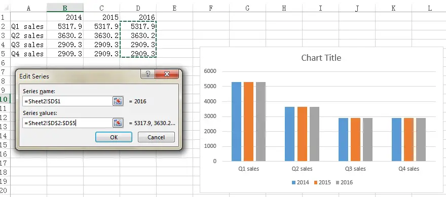
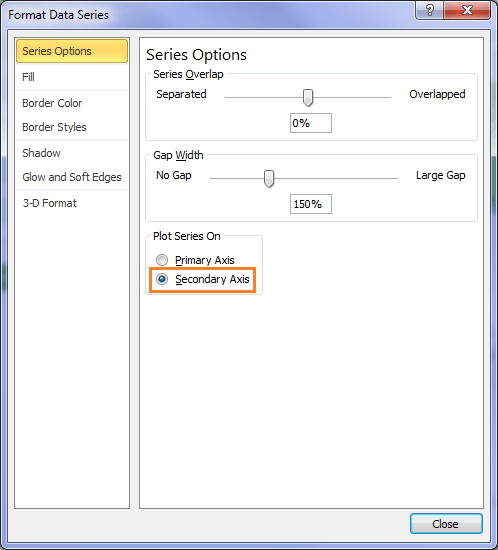
Adding second set of data labels - Excel Help Forum Re: Adding second set of data labels. The chart links to workbooks on your hard drive, not to the data in the sheet. The secondary axis can only be shown when there is a series plotting on the secondary axis. Both your series are plotted on the first axis. You need to select the COUNT OF PARTS series, format it and send it to the secondary axis.

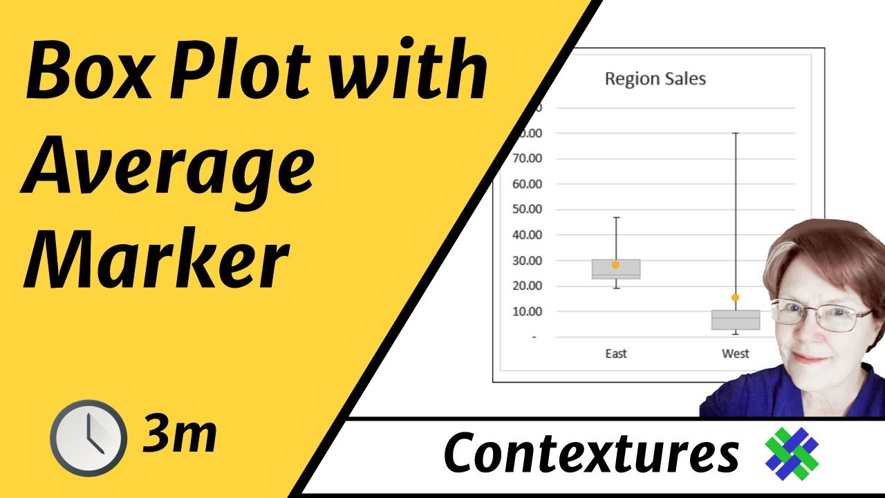
Add Average Marker to Excel Box Plot - Box and Whisker Chart - YouTube

Improve your X Y Scatter Chart with custom data labels May 06, 2021 · Thank you for your Excel 2010 workaround for custom data labels in XY scatter charts. It basically works for me until I insert a new row in the worksheet associated with the chart. Doing so breaks the absolute references to data labels after the inserted row and Excel won't let me change the data labels to relative references.

How to Add Data Labels in an Excel Chart in Excel 2010 - YouTube

How to Add Labels to Show Totals in Stacked Column Charts in Excel Press the Ok button to close the Change Chart Type dialog box. The chart should look like this: 8. In the chart, right-click the "Total" series and then, on the shortcut menu, select Add Data Labels. 9. Next, select the labels and then, in the Format Data Labels pane, under Label Options, set the Label Position to Above. 10.

Basic Excel Chart Formatting - MS Excel Charting Tutorial Part 4 | Vertical Horizons

Apply Custom Data Labels to Charted Points - Peltier Tech With a chart selected, click the Add Labels ribbon button (if a chart is not selected, a dialog pops up with a list of charts on the active worksheet). A dialog pops up so you can choose which series to label, select a worksheet range with the custom data labels, and pick a position for the labels.

How to create Pie of Pie or Bar of Pie chart in Excel

How to Add Data Labels to an Excel 2010 Chart - dummies On the Chart Tools Layout tab, click Data Labels→More Data Label Options. The Format Data Labels dialog box appears. You can use the options on the Label Options, Number, Fill, Border Color, Border Styles, Shadow, Glow and Soft Edges, 3-D Format, and Alignment tabs to customize the appearance and position of the data labels.

How to Make Excel Charts More Intuitive by Adding Data Labels and Tables - Data Recovery Blog

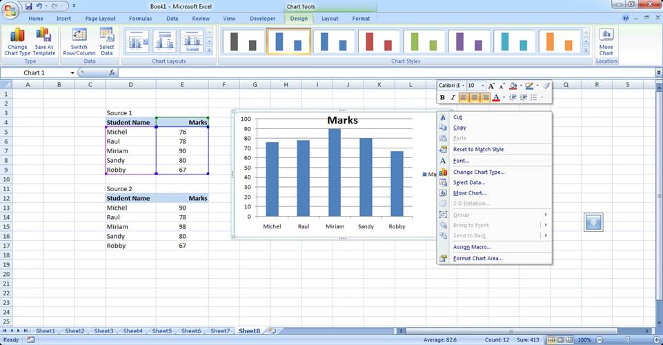
Add a data series to your chart - support.microsoft.com Right-click the chart, and then choose Select Data. The Select Data Source dialog box appears on the worksheet that contains the source data for the chart. Leaving the dialog box open, click in the worksheet, and then click and drag to select all the data you want to use for the chart, including the new data series.

Enable or Disable Excel Data Labels at the click of a button - How To - PakAccountants.com

Create Dynamic Chart Data Labels with Slicers - Excel Campus Feb 10, 2016 · This is because Excel 2010 does not contain the Value from Cells feature. Jon Peltier has a great article with some workarounds for applying custom data labels. This includes using the XY Chart Labeler Add-in, which is a free download for Windows or Mac. Step 6: Setup the Pivot Table and Slicer. The final step is to make the data labels ...

Pivot table row labels in separate columns • AuditExcel.co.za

How to Use Cell Values for Excel Chart Labels Select the chart, choose the "Chart Elements" option, click the "Data Labels" arrow, and then "More Options." Uncheck the "Value" box and check the "Value From Cells" box. Select cells C2:C6 to use for the data label range and then click the "OK" button. The values from these cells are now used for the chart data labels.

Excel clustered column chart - Access-Excel.Tips

Adding Data Labels to Your Chart (Microsoft Excel) - tips To add data labels, follow these steps: Activate the chart by clicking on it, if necessary. Choose Chart Options from the Chart menu. Excel displays the Chart Options dialog box. Make sure the Data Labels tab is selected. (See Figure 1.) The left side of the dialog box shows the different types of data labels you can choose.

32 What Is A Data Label In Excel - Labels Design Ideas 2020

How to add or move data labels in Excel chart? - ExtendOffice To add or move data labels in a chart, you can do as below steps: In Excel 2013 or 2016. 1. Click the chart to show the Chart Elements button .. 2. Then click the Chart Elements, and check Data Labels, then you can click the arrow to choose an option about the data labels in the sub menu.See screenshot:

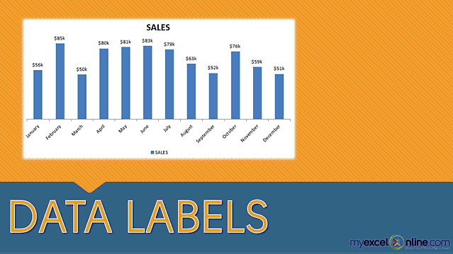
Adding Data Labels To An Excel Chart | MyExcelOnline

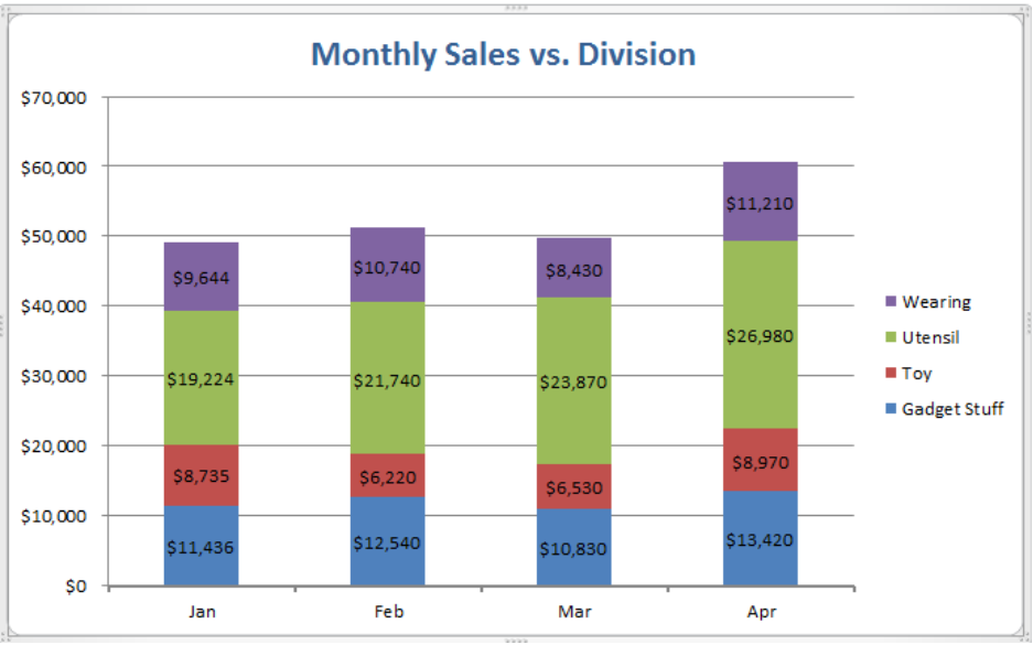
How to Add Total Data Labels to the Excel Stacked Bar Chart Apr 03, 2013 · Step 4: Right click your new line chart and select “Add Data Labels” Step 5: Right click your new data labels and format them so that their label position is “Above”; also make the labels bold and increase the font size. Step 6: Right click the line, select “Format Data Series”; in the Line Color menu, select “No line”

Excel Custom Chart Labels • My Online Training Hub

Chart.ApplyDataLabels method (Excel) | Microsoft Docs For the Chart and Series objects, True if the series has leader lines. Pass a Boolean value to enable or disable the series name for the data label. Pass a Boolean value to enable or disable the category name for the data label. Pass a Boolean value to enable or disable the value for the data label.

How to Add Data Labels in Excel - Excelchat | Excelchat

Add a DATA LABEL to ONE POINT on a chart in Excel Click on the chart line to add the data point to. All the data points will be highlighted. Click again on the single point that you want to add a data label to. Right-click and select ' Add data label ' This is the key step! Right-click again on the data point itself (not the label) and select ' Format data label '.

Excel Gantt Chart - Free Excel Templates

Use a screen reader to add a title, data labels, and a legend to a ... Select the chart that you want to work with. To open the Add Chart Element menu, press Alt+J, C, A. Select the type of title you want to add: To add a chart title, press C. The focus moves to the Chart title list. Do one of the following: To add a title above the chart, press A, type a title, and then press Enter.

Basic Excel Chart Formatting - MS Excel Charting Tutorial Part 4 | Vertical Horizons

How to Add Data Labels in Excel - Excelchat | Excelchat After inserting a chart in Excel 2010 and earlier versions we need to do the followings to add data labels to the chart; Click inside the chart area to display the Chart Tools. Figure 2. Chart Tools Click on Layout tab of the Chart Tools. In Labels group, click on Data Labels and select the position to add labels to the chart. Figure 3.