38 excel chart add data labels to all series

Add a data series to your chart - support.microsoft.com In that case, you can enter the new data for the chart in the Select Data dialog box. Add a data series to a chart on a chart sheet. On the worksheet, in the cells directly next to or below the source data of the chart, type the new data and labels you want to add. Custom Chart Data Labels In Excel With Formulas Select the chart label you want to change. In the formula-bar hit = (equals), select the cell reference containing your chart label's data. In this case, the first label is in cell E2. Finally, repeat for all your chart laebls. If you are looking for a way to add custom data labels on your Excel chart, then this blog post is perfect for you.

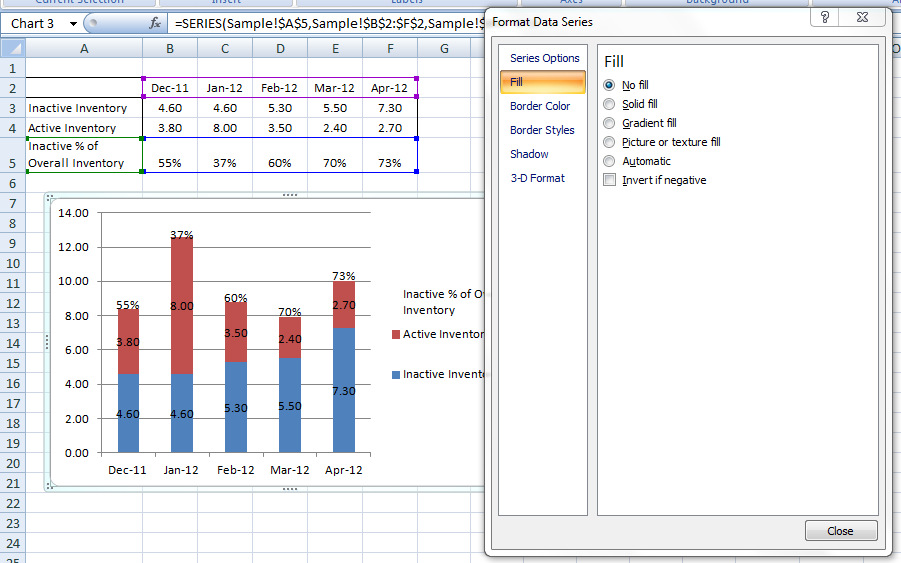
How to Add Total Data Labels to the Excel Stacked Bar Chart Apr 03, 2013 · Step 4: Right click your new line chart and select “Add Data Labels” Step 5: Right click your new data labels and format them so that their label position is “Above”; also make the labels bold and increase the font size. Step 6: Right click the line, select “Format Data Series”; in the Line Color menu, select “No line” Step 7 ...

Excel chart add data labels to all series

Adding Data Labels to a Chart Using VBA Loops - Wise Owl Making Sure the Chart has Data Labels. Before we can set the text that appears in the data labels, we need to make sure that the data series actually has labels ready for us to change! One way to do this is by manually adding data labels to the chart within Excel, but we're going to achieve the same result in a single line of code. To do this ... excel - Change format of all data labels of a single series at once ... A quick way to solve this is to: Go to the chart and left mouse click on the 'data series' you want to edit. Click anywhere in formula bar above. Don't change anything. Click the 'tick icon' just to the left of the formula bar. Go straight back to the same data series and right mouse click, and choose add data labels. Multiple Time Series in an Excel Chart - Peltier Tech Aug 12, 2016 · Start by selecting the monthly data set, and inserting a line chart. Excel has detected the dates and applied a Date Scale, with a spacing of 1 month and base units of 1 month (below left). Select and copy the weekly data set, select the chart, and use Paste Special to add the data to the chart (below right).

Excel chart add data labels to all series. Comparison Chart in Excel | Adding Multiple Series Under Same … This window helps you modify the chart as it allows you to add the series (Y-Values) as well as Category labels (X-Axis) to configure the chart as per your need. Under Legend Entries (Series) inside the Select Data Source window, you need to select the sales values for the year 2018 and year 2019. Follow the step below to get this done. Change the labels in an Excel data series | TechRepublic Click the Chart Wizard button in the Standard toolbar. Click Next. Click the Series tab. Click the Window Shade button in the Category (X) Axis. Labels box. Select B3:D3 to select the labels in ... chandoo.org › wp › change-data-labels-in-chartsHow to Change Excel Chart Data Labels to Custom Values? May 05, 2010 · First add data labels to the chart (Layout Ribbon > Data Labels) Define the new data label values in a bunch of cells, like this: Now, click on any data label. This will select “all” data labels. Now click once again. At this point excel will select only one data label. How to add or move data labels in Excel chart? - ExtendOffice In Excel 2013 or 2016. 1. Click the chart to show the Chart Elements button . 2. Then click the Chart Elements, and check Data Labels, then you can click the arrow to choose an option about the data labels in the sub menu. See screenshot: In Excel 2010 or 2007. 1. click on the chart to show the Layout tab in the Chart Tools group. See ...

How to Change Excel Chart Data Labels to Custom Values? May 05, 2010 · First add data labels to the chart (Layout Ribbon > Data Labels) Define the new data label values in a bunch of cells, like this: Now, click on any data label. This will select “all” data labels. Now click once again. At this point excel will select only one data label. Excel Charts: Dynamic Label positioning of line series - XelPlus Select your chart and go to the Format tab, click on the drop-down menu at the upper left-hand portion and select Series "Actual". Go to Layout tab, select Data Labels > Right. Right mouse click on the data label displayed on the chart. Select Format Data Labels. Under the Label Options, show the Series Name and untick the Value. Add or remove data labels in a chart - support.microsoft.com Depending on what you want to highlight on a chart, you can add labels to one series, all the series (the whole chart), or one data point. Add data labels. You can add data labels to show the data point values from the Excel sheet in the chart. This step applies to Word for Mac only: On the View menu, click Print Layout. › charts › dynamic-chart-dataCreate Dynamic Chart Data Labels with Slicers - Excel Campus Feb 10, 2016 · You basically need to select a label series, then press the Value from Cells button in the Format Data Labels menu. Then select the range that contains the metrics for that series. Click to Enlarge. Repeat this step for each series in the chart. If you are using Excel 2010 or earlier the chart will look like the following when you open the file.

Excel charts: add title, customize chart axis, legend and data labels ... Depending on where you want to focus your users' attention, you can add labels to one data series, all the series, or individual data points. Click the data series you want to label. To add a label to one data point, click that data point after selecting the series. Click the Chart Elements button, and select the Data Labels option. Create Dynamic Chart Data Labels with Slicers - Excel Campus Feb 10, 2016 · You basically need to select a label series, then press the Value from Cells button in the Format Data Labels menu. Then select the range that contains the metrics for that series. Click to Enlarge. Repeat this step for each series in the chart. If you are using Excel 2010 or earlier the chart will look like the following when you open the file. › excel › how-to-add-total-dataHow to Add Total Data Labels to the Excel Stacked Bar Chart Apr 03, 2013 · Step 4: Right click your new line chart and select “Add Data Labels” Step 5: Right click your new data labels and format them so that their label position is “Above”; also make the labels bold and increase the font size. Step 6: Right click the line, select “Format Data Series”; in the Line Color menu, select “No line” Step 7 ... Add a Data Series to Chart - Excel & Google Sheets Add the additional series to the table. Right click on graph. Select Data Range. 4. Select Add Series. 5. Click box to Select a Data Range. 6. Highlight the new Series Dataset and click OK.

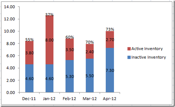
Excel Dashboard Templates How-to Put Percentage Labels on Top of a Stacked Column Chart - Excel ...

How to set all data labels with Series Name at once in an Excel 2010 chart chart series data labels are set one series at a time. If you don't want to do it manually, you can use VBA. Something along the lines of Sub setDataLabels () ' ' sets data labels in all charts ' Dim sr As Series Dim cht As ChartObject ' With ActiveSheet For Each cht In .ChartObjects For Each sr In cht.Chart.SeriesCollection sr.ApplyDataLabels

Do My Excel Blog: How to design a multiple clustered bar chart series in Excel

Chart.ApplyDataLabels method (Excel) | Microsoft Docs For the Chart and Series objects, True if the series has leader lines. ShowSeriesName: Optional: Variant: Pass a Boolean value to enable or disable the series name for the data label. ShowCategoryName: Optional: Variant: Pass a Boolean value to enable or disable the category name for the data label. ShowValue: Optional: Variant

Understanding Excel Chart Data Series, Data Points, and Data Labels

› documents › excelHow to add data labels from different column in an Excel chart? This method will guide you to manually add a data label from a cell of different column at a time in an Excel chart. 1. Right click the data series in the chart, and select Add Data Labels > Add Data Labels from the context menu to add data labels. 2. Click any data label to select all data labels, and then click the specified data label to ...

How-to Use Data Labels from a Range in an Excel Chart - Excel Dashboard Templates

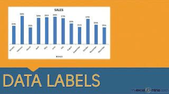
Adding Data Labels To An Excel Chart | MyExcelOnline Depending on what you want to highlight on a chart, you can add labels to one series, all the series (the whole chart), or one data point. In our example below, I add a Data Label to a column chart and then I format the data label using CTRL+1.

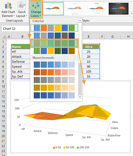
Surface Chart in Excel

Excel chart changing all data labels from value to series name ... By selecting chart then from layout->data labels->more data labels options ->label options ->label contains-> (select)series name, I can only get one series name replacing its respective label values. For more than hundred series stacked in columns i want them all to be changed at once, is there any way out? why it does not change them all at once?

Excel Dashboard Templates How-to Put Percentage Labels on Top of a Stacked Column Chart - Excel ...

Dynamically Label Excel Chart Series Lines - My Online Training Hub Step 4: Add the Labels. Excel 2013/2016 Click the + icon beside the chart as shown below (Note: for Excel 2007/2010 go to Layout tab) Data Labels. More Options. This will open the Format Data Labels pane/dialog box where you can choose 'Series Name' and label position; Right, as shown in the image below as shown in the image below for Excel ...

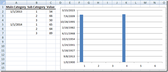
Fixing Your Excel Chart When the Multi-Level Category Label Option is Missing. - Excel Dashboard ...

support.microsoft.com › en-us › officeAdd or remove data labels in a chart - support.microsoft.com Click the data series or chart. To label one data point, after clicking the series, click that data point. In the upper right corner, next to the chart, click Add Chart Element > Data Labels. To change the location, click the arrow, and choose an option. If you want to show your data label inside a text bubble shape, click Data Callout.

30 What Is A Data Label In Excel - Labels Database 2020

Adding series labels - Excel Help Forum Re: Adding series labels. Here is a small example. Main data is 200 points. I copied the data set and sorted on x then y values. Only the top 10 points are plotted and have data labels enabled. I used a dynamic named range so changing the value in C1 will alter the number of data labels displayed. Attached Files.

How to Customize Your Excel Pivot Chart Data Labels - dummies

How to add data labels from different column in an Excel chart? This method will guide you to manually add a data label from a cell of different column at a time in an Excel chart. 1. Right click the data series in the chart, and select Add Data Labels > Add Data Labels from the context menu to add data labels. 2. Click any data label to select all data labels, and then click the specified data label to ...

How to Make Charts and Graphs in Excel | Smartsheet

Formal ALL data labels in a pivot chart at once Hi AaronSchmid ，. I go through the post, as per the article: Change the format of data labels in a chart, you may select only one data labels to format it. However, you may change the location of the data labels all at once, as you can see in screenshot below: I would suggest you vote for or leave your comments in the thread: Format Data ...

How to Change Excel Chart Data Labels to Custom Values?

› data-series-data-points-dataUnderstanding Excel Chart Data Series, Data Points, and Data ... Sep 19, 2020 · Data Series: A group of related data points or markers that are plotted in charts and graphs. Examples of a data series include individual lines in a line graph or columns in a column chart. When multiple data series are plotted in one chart, each data series is identified by a unique color or shading pattern.

Excel Dashboard Templates Fixing Your Excel Chart When the Multi-Level Category Label Option is ...

How to Add Data Labels in Excel - Excelchat | Excelchat After inserting a chart in Excel 2010 and earlier versions we need to do the followings to add data labels to the chart; Click inside the chart area to display the Chart Tools. Figure 2. Chart Tools Click on Layout tab of the Chart Tools. In Labels group, click on Data Labels and select the position to add labels to the chart. Figure 3.

Format Number Options for Chart Data Labels in Excel 2011 for Mac

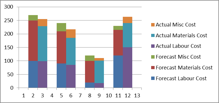
How to Add Labels to Show Totals in Stacked Column Charts in Excel Press the Ok button to close the Change Chart Type dialog box. The chart should look like this: 8. In the chart, right-click the "Total" series and then, on the shortcut menu, select Add Data Labels. 9. Next, select the labels and then, in the Format Data Labels pane, under Label Options, set the Label Position to Above. 10.

Adding Data Labels To An Excel Chart | Free Microsoft Excel Tutorials

Excel Chart with Positive and Negative Numbers Right-click on any data series and choose Format Data Series… from the context menu that pops up: In the Format Data Series pane, adjust the Series Overlap to 0% and the Gap Width to 30% or another percentage that suits your situation. The chart now looks as follows: Right-click on the negative series and click Add Data Labels >> Add Data Labels:

Step-by-step tutorial on creating clustered stacked column bar charts (for free) | Excel Help HQ

Add / Move Data Labels in Charts - Excel & Google Sheets Double Click Chart Select Customize under Chart Editor Select Series 4. Check Data Labels 5. Select which Position to move the data labels in comparison to the bars. Final Graph with Google Sheets After moving the dataset to the center, you can see the final graph has the data labels where we want.

30 How To Add Label To Excel Chart - Labels Database 2020

Excel charts: how to move data labels to legend - Microsoft Tech Community You can't do that, but you can show a data table below the chart instead of data labels: Click anywhere on the chart. On the Design tab of the ribbon (under Chart Tools), in the Chart Layouts group, click Add Chart Element > Data Table > With Legend Keys (or No Legend Keys if you prefer)

Share :